k-means Clustering

4/27/23

Housekeeping

• Project plans of analysis due Sunday!

Unsupervised learning

What is unsupervised learning?

• Shifting gears: instead of supervised learning (e.g. regression and classification), we will now turn to unsupervised learning

• We only observe the features \(X_{1}, X_{2},\ldots, X_{p}\)

  • We do not care about prediction because we have no response \(Y\)!

  • For this reason, the \(X_{1}, X_{2},\ldots, X_{p}\) are often referred to as “features” in unsupervised learning, rather than “predictors”

• Example: a search engine might choose which search results to display to a particular individual based on the click histories of other individuals with similar search patterns

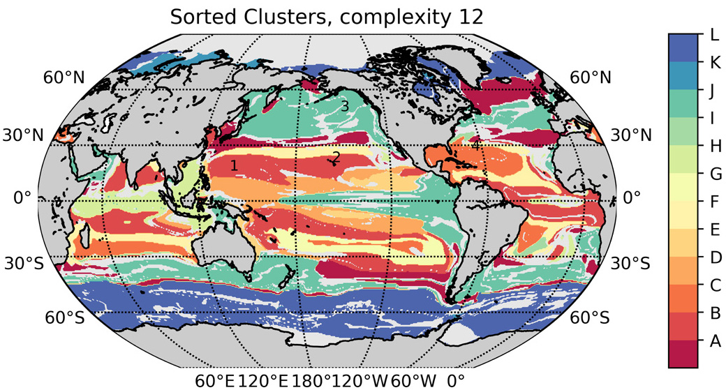
Real-life example

Marine eco-provinces

Unsupervised learning goals

• Discover interesting things about the predictors/features

  • Can we discover subgroups among the variables or among the observations?

  • Is there an informative way to visualize the data?

• Two common methods:

  • Clustering: broad class of methods to discover unknown subgroups in your data

  • Principal components analysis (PCA): a tool used for data visualization or data pre-processing, often before supervised techniques are applied

    • PCA is beyond the scope of this course (but you can try using it for your final project if you understand eigenvectors!)

Challenges

• Subjective; no clearly defined goal for analysis

• How to assess results obtained? No way to validate without a true response!

• Despite challenges, unsupervised learning methods are of growing importance

Clustering

• We want to find subgroups or clusters in a data set

• This means separating observations into distinct groups such that:

  • observations with each group are similar

  • observation across groups are different

• How to define “similar” and “different”?

• Two main methods: K-means clustering and hierarchical clustering

  • Apologies for another K!

K-Means clustering: introduction

General idea

• We seek to partition/divide the observations into a pre-specified number of clusters \(K\)

• These clusters are distinct and non-overlapping

• Just like in \(k\)-fold CV or KNN, we first specify \(K\).

  • Then the algorithm will assign each observation in the dataset to exactly one of the \(K\) clusters

Example 1: US Arrests

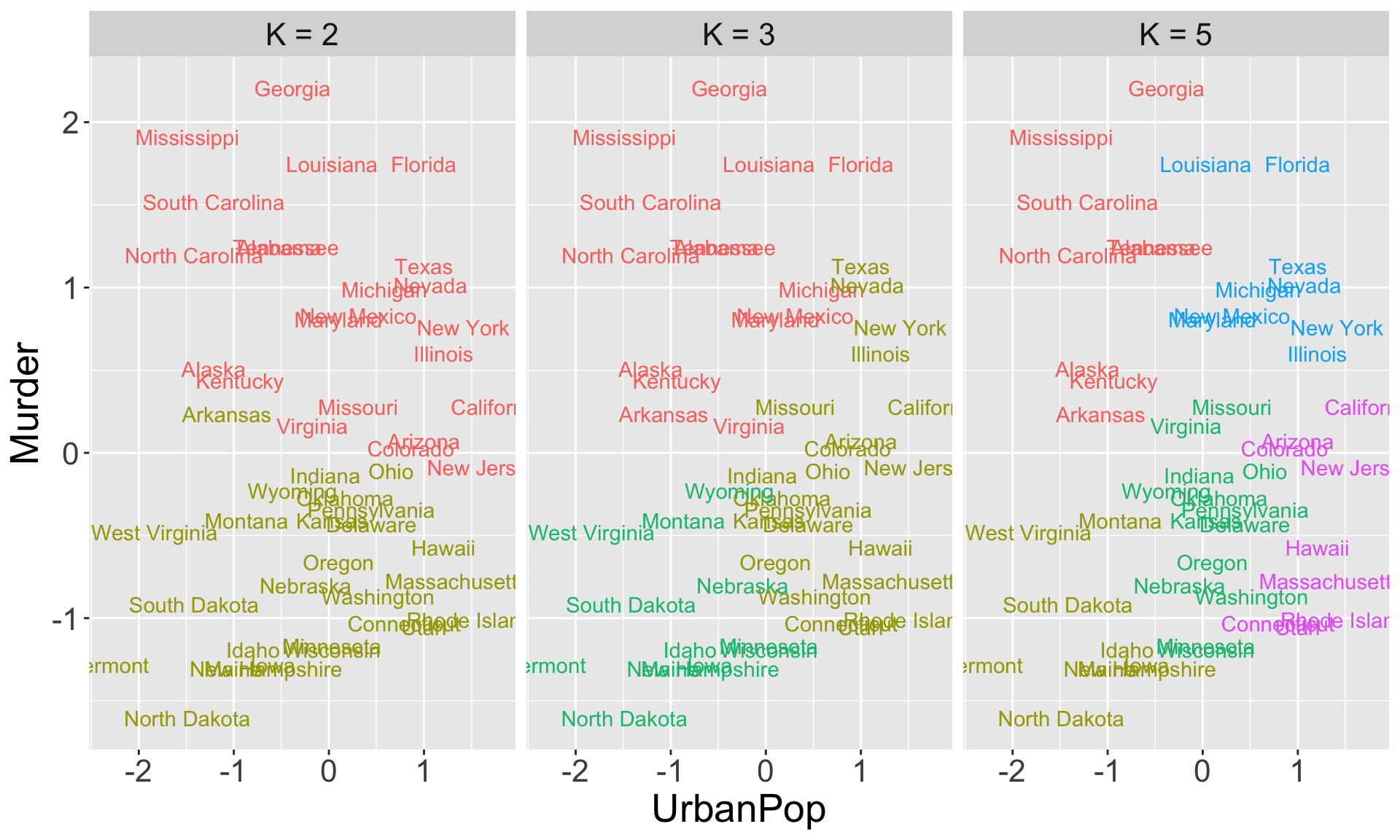
• USArrests data in R contains statistics about arrests per 100,000 residents for \(\color{blue}{\text{Murder}}\) in each of the 50 US states in 1973. Also given is the percent of the population living in urban areas \((\color{blue}{\text{UrbanPop}})\).

• In the following slide, I apply \(K\)-means clustering with different values of \(K\) to group the observations (states)

• Color of each observation indicates the cluster to which each state was assigned (coloring is arbitrary)

Example 1: US Arrests

Example 2: simulated data

• Simulated data with \(n = 60\) observations in 3-dimensional space, with three true clusters

• The following plots show the results of applying \(K\)-means clustering with different \(K\)

  • Color corresponds to cluster

Example 2: 2-means

Example 2: 3-means

Example 2: 5-means

K-means clustering: details

Notation

• Procedure results from simple and intuitive mathematical problem. We will start with notation

• Let \(C_{1}, \ldots, C_{K}\) be the sets containing the indices of the observation in each cluster. These sets satisfy two properties:

  1. \(C_{1} \cup C_{2} \cup \ldots \cup C_{K} = \{1, \ldots, n\}\), i.e. each observation belong to at least one of the \(K\) clusters

  2. \(C_{k} \cap C_{k'} = \emptyset\) for all \(k \neq k'\), i.e. the clusters are non-overlapping

• For example, if the 10-th observation is in the second cluster, then \(10 \in C_{2}\)

  • More generally: if observation \(i\) is in the \(k\)-th cluster, then \(i \in C_{k}\)

Within-cluster-variation

• Good clustering is at the heart of \(K\)-means clustering procedure: we want the within-cluster variation to be as small as possible

• Let \(\text{WCV}(C_{k})\) denote the within-cluster variation for cluster \(C_{k}\). It tells us the amount by which observations within a cluster are different from each other

• \(K\)-means clustering solves the problem: \[\min_{C_{1}, \ldots, C_{K}}\left\{\sum_{k=1}^{K}\text{WCV}(C_{k}) \right\}\]

• What does this mean in words?

  • This is called the “objective”

Defining WCV

Most common choice of WCV is (pairwise) squared Euclidean distance:

\[\begin{align*} \text{WCV}(C_{k}) &= \frac{1}{|C_{k}|} \sum_{i, i' \in C_{k}} d(\mathbf{x}_{i}, \mathbf{x}_{i'})^2\\ &= \frac{1}{|C_{k}|} \sum_{i, i' \in C_{k}} \sum_{j=1}^{p} (x_{ij} - x_{i'j})^2 \end{align*} \] where \(|C_{k}|\) is the number of observations in the \(k\)-th cluster and \(d()\) is the usual Euclidean distance function we are familiar with

• In words: WCV for the \(k\)-th cluster is the sum of all of the pairwise squared Euclidean distances between the observations in the \(k\)-th cluster, divided by the total number of observations in that cluster.

Optimization problem

Combining the the objective with our definition of WCV, \(K\)-means clustering tries to solve the following problem:

\[\min_{C_{1}, \ldots, C_{K}}\left\{\sum_{k=1}^{K} \frac{1}{|C_{k}|} \sum_{i, i' \in C_{k}} d(\mathbf{x}_{i}, \mathbf{x}_{i'}) \right\}\]

• So, we need an algorithm to solve this problem; i.e. find the set of clusters \(C_{1}, \ldots, C_{k}\) that minimize this function!

• We will learn one possible algorithm for solving this optimization problem

Algorithm

0. Choose \(K\)

1. Randomly assign each observation to one of the \(K\) clusters. This is how we initialize the cluster assignments.

2. Iterate the following until the cluster assignments stop changing:

   1. For each cluster \(k = 1,\ldots, K\), compute the cluster centroid.

   2. Assign each observation to the cluster whose centroid is closest, where we determine “close” using Euclidean distance

Centroids

• Each cluster has a centroid that changes at every iteration

• The \(k\)-th cluster centroid is the vector of the \(p\)-feature means for observation in \(C_{k}\)

• E.g. we have two features X1 and X2, and each observation (row) is currently in cluster 1 or 2.

  X1 X2 cluster
1  1  6       1
2  3  5       1
3  4  2       2
4  1  3       2
5  2  3       2
6  5  1       2

• What are the centroids of each cluster?

# A tibble: 2 × 3
  cluster_centroid    X1    X2
             <int> <dbl> <dbl>
1                1     2  5.5 
2                2     3  2.25

In-class example

Important implementation concerns!

• This algorithm is not guaranteed to solve the minimization problem exactly

• There are almost \(K^n\) ways to partition all \(n\) observations into \(K\) clusters

• The algorithm on previous slide provides a local optimum, i.e. a pretty good solution to the optimization problem!

• Because the algorithm finds a local optimum, our results will depend on the initial cluster assignments in Step 1

  • Therefore, it is important to run the algorithm multiple times using different random initializations

  • Then select the best solution (i.e. the one with smallest objective value \(\sum_{k=1}^{K}\text{WCV}(C_{k})\))

Example 3: Simulated data

• Generated \(n=50\) observations with two features, evenly split between two true clusters

• Perform K-means clustering performed four times on the same data with \(K = 3\), each time with different random initialization.

• Above each plot is the value of the objective

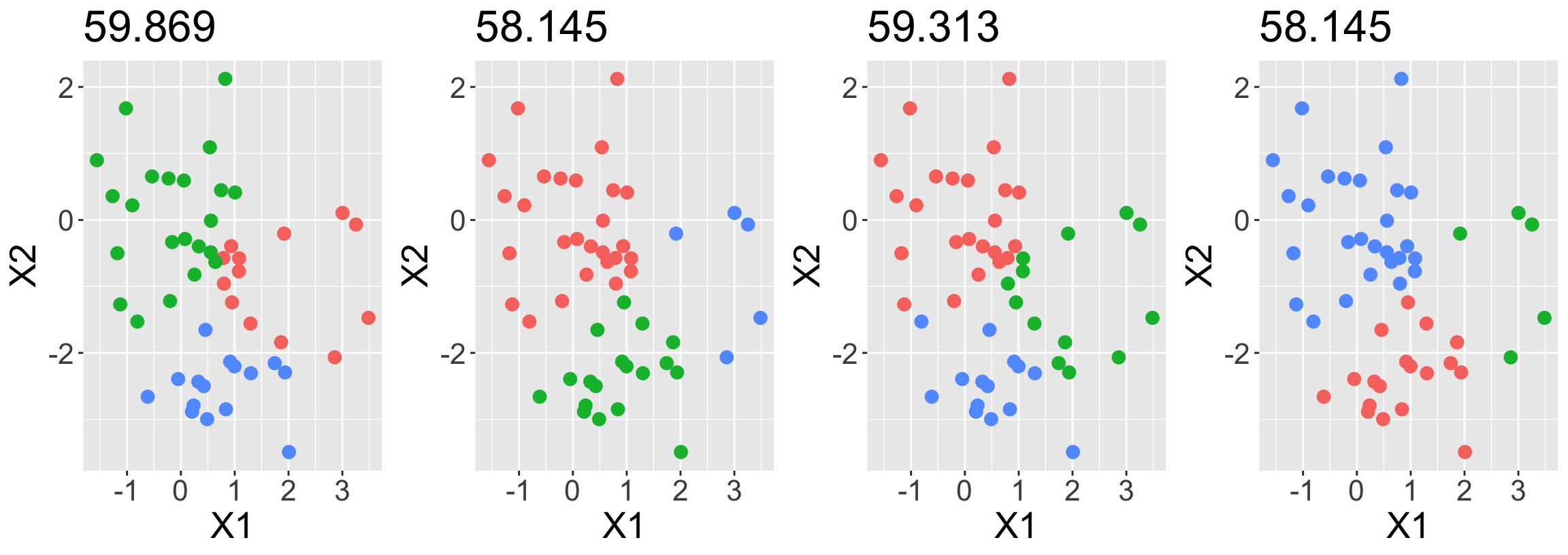
• Three different local optima were obtained (three unique objective values)

• One of the local optima resulted in a smaller value of the objective, and therefore provides better separation between the clusters

  • Two of the initializations results in ties for best solution, with objective value of 58.145

Example 4: seeds data

• Recall the seeds data with three varieties: Kama, Rosa, and Canadian

• Run \(K\)-means with \(K = 3\), using features compactness and area

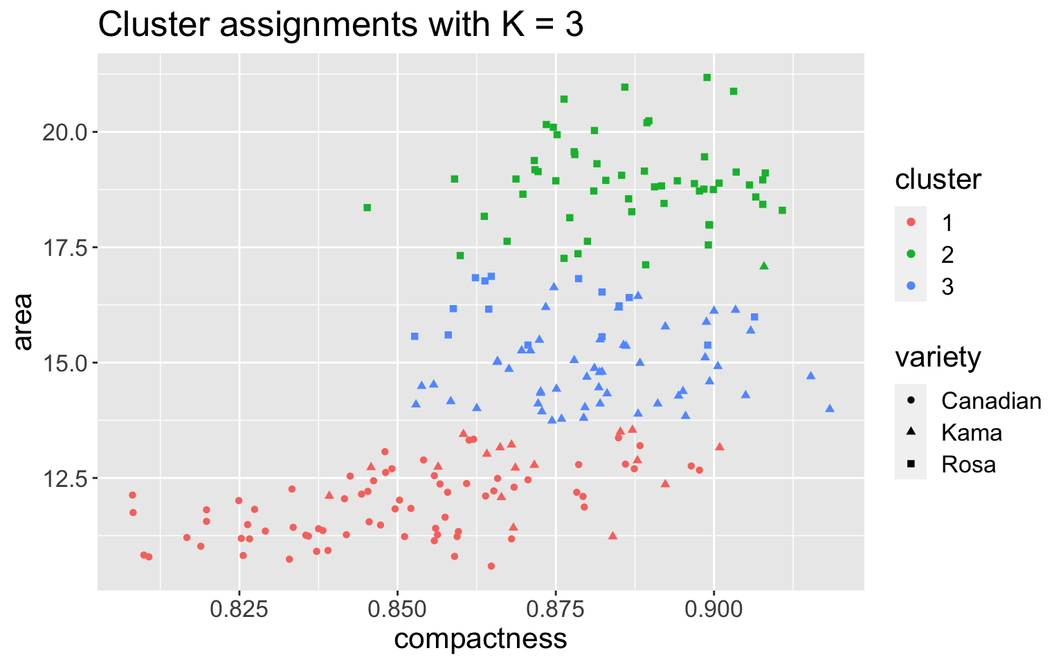
• If I didn’t know there were truly three classes, how would I choose \(K\)?

Elbow method

• Popular heuristic to determine the optimal value of \(K\)

• Fit \(K\)-means several times with different \(K\) values, and plot the objective values against the number of clusters \(K\)

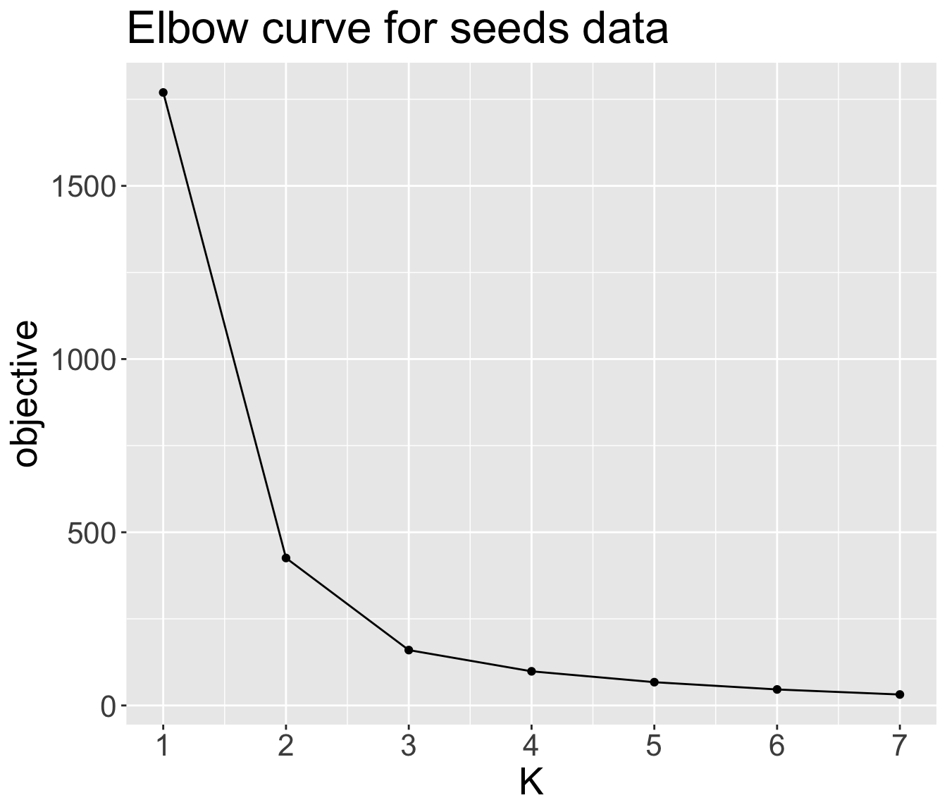
• Graph will (hopefully) rapidly change at a point and thus create the elbow shape.

  • The \(K\) value where elbow “bends” and begins to run parallel to x-axis is taken to be optimal

  • What is the optimal \(K\) for the seeds data?

• Unfortunately, it is not always obvious where the curve bends

Live code

Where k-means fails

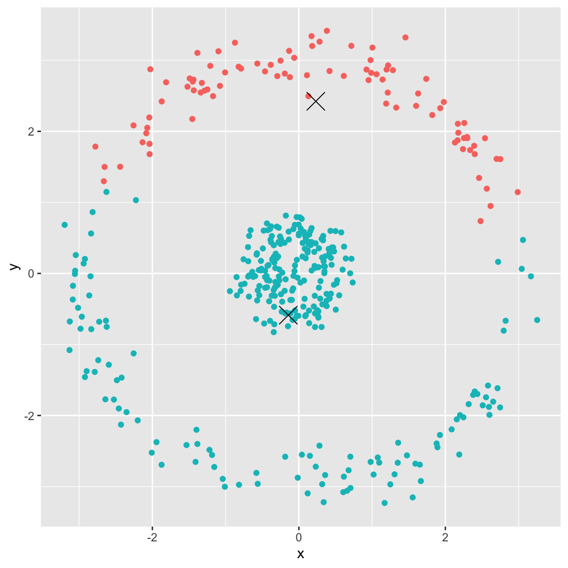
Example 5: spherical data

Generated the following data:

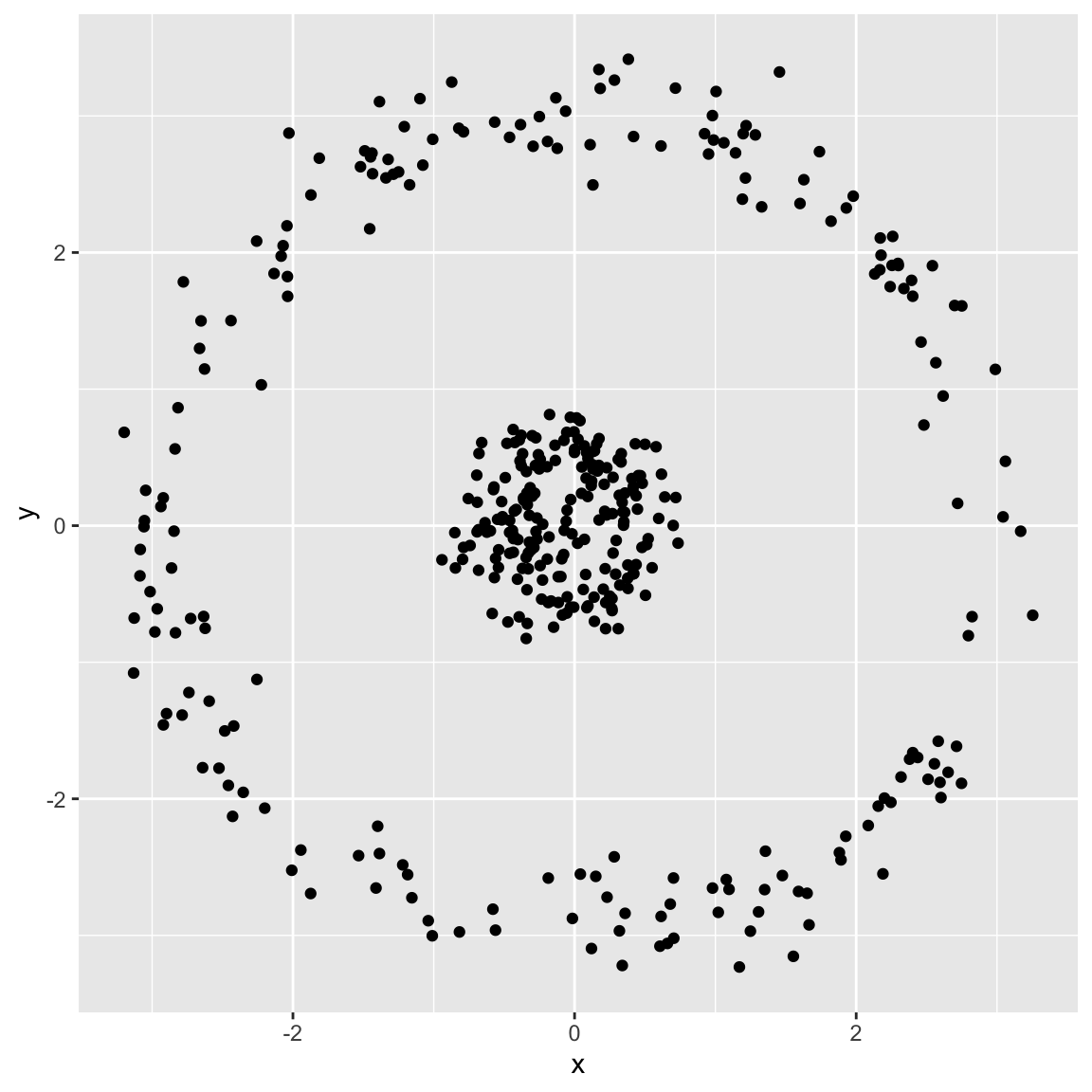
• Running \(K\)-means with \(K=2\)

Example 6: differing densities

Generated three clusters with differing densities (number of observations), \(n = 20, 100, 500\)

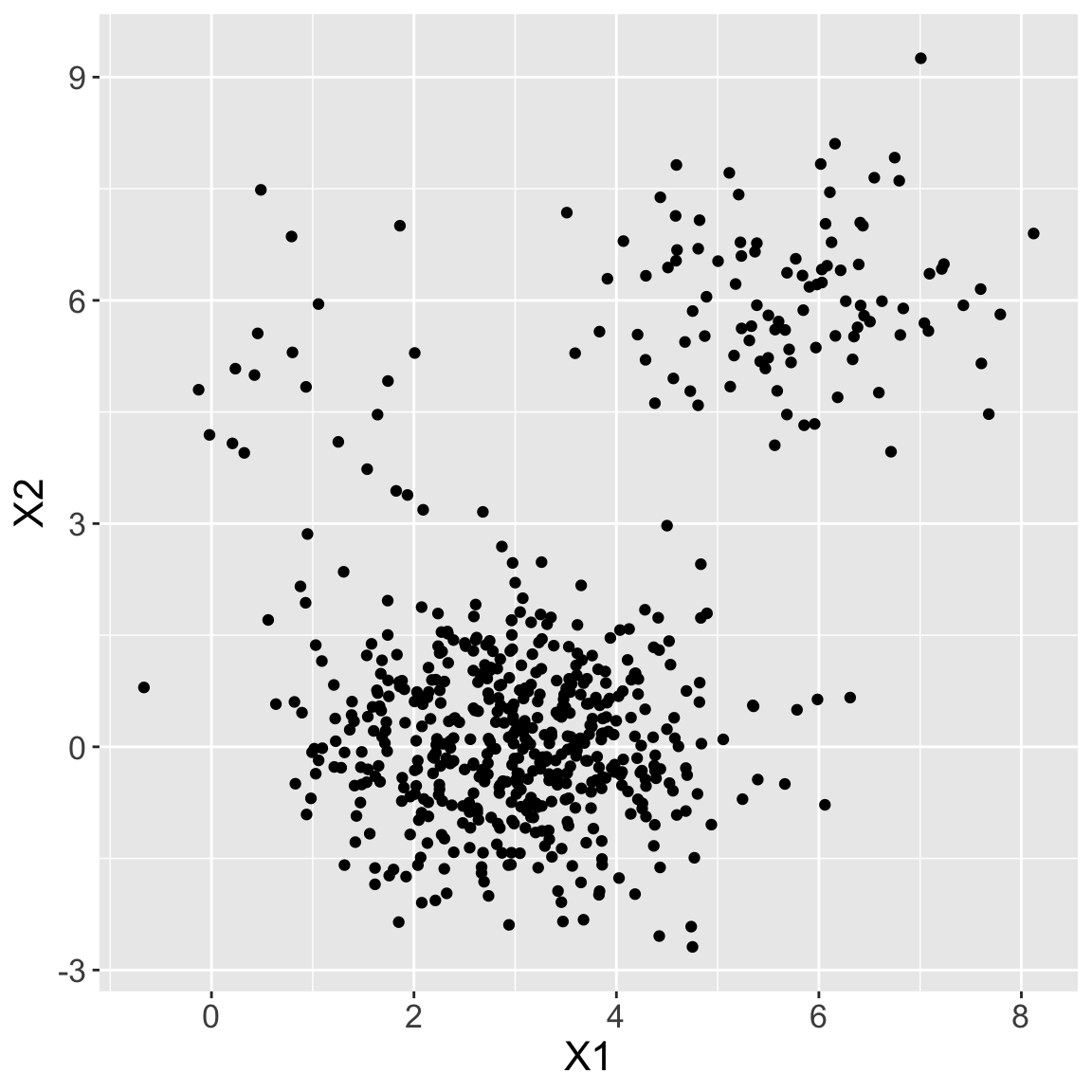
• Fit \(K\)-means with \(K = 3\). What’s happening?

Similar model: K-medoids

• \(K\)-medoids: very similar to \(K\)-means clustering

  • \(K\)-means chooses centers of clusters as the average between the points in the cluster, thus the centroid is usually not one of the observed points

  • \(K\)-medoids chooses one of the observation points to be the center

  • Like mean vs. median

• Allows for greater interpretability of the center clusters compared to \(K\)-means

K-medoids vs K-means

• \(K\)-medoids can be used with arbitrary dissimilarity measures, whereas \(K\)-means generally requires Euclidean distance for efficient solutions

• \(K\)-medoids minimizes the sum of pairwise dissimilarities, whereas \(K\)-means attempts to minimize sum of (squared) Euclidean distances

  • Thus, \(K\)-medoids is more robust to noise and outliers

Better initialization?

Is randomly initializing the most intelligent way to run the algorithm?

• What are some possible issues of randomly initializing?

• Minimizing the objective (smallest \(\sum_{k=1}^{K}\text{WCV}(C_{k})\)) gets at the goal of observations within a cluster being as similar as possible

  • But it doesn’t do much for the goal of making sure the each cluster is distinct

• How might we encode this notion of “far away” clusters when we initialize?

  • More commonly used initialization method: k-means++

Summary

Drawbacks

• Does not take into account the different densities of each cluster

• Number of clusters in the data \(K\) is fixed and assumed known

• Relies on minimizing within-cluster variance (i.e. sum of squared Euclidean distance), which is not always appropriate

  • Does not handle categorical features well

• Lack of interpretation of clusters

• Can be slow for large \(n\)

Considerations

• Should the features be standardized?

  • This is always a question when distances are involved!

• What should \(K\) be?

• How do we validate the clusters we obtained?

  • Are we truly discovering subgroups, or are we simply clustering the noise?

• Do all observations belong in a cluster? Or are some actually “outliers”

• Clustering methods generally not robust to small changes in data

Recommendations

• Recommend performing clustering with different choices of \(K\), and looking to see if/which patterns consistently appear

  • Elbow method

• Because clustering not robust, maybe we consider clustering subsets of the data

• Caution: be careful about how the results of a clustering analysis are reported. These results should not be taken as the absolute truth about a data set!!!