Classification & Logistic Regression
4/4/23
Housekeeping
How was the midterm??
- Grades should be uploaded by end of week!
Please e-mail me about project partners by this Saturday!
Categorical responses
Classification
Up until now, we have focused on quantitative responses \(y_{i}\)
What happens when \(y_{i}\) is qualitative? Examples include:
Medical diagnosis: \(\mathcal{C} = \{\text{yes}, \text{no}\}\)
Education level: \(\mathcal{C} = \{\text{high school}, \text{college}, \text{graduate}\}\)
Each category in \(\mathcal{C}\) is also known as a label
In this setting, we want our model to be a classifier, i.e. given predictors \(X\), predict a label from the pool of all possible categories \(\mathcal{C}\)
Classification
Model: \(y_{i} = f(x_{i}) + \epsilon_{i}\)
We will still have to estimate \(f\) with a \(\hat{f}\)
\(\hat{y}_{i}\) is the predicted class label for observation \(i\) using estimate \(\hat{f}\)
How to assess model accuracy? Error is more intuitive in classification: we make an error if we predict the incorrect label, and no error otherwise
Classification error
This can be represented using an indicator variable or function \(\mathbf{1}(y_{i} = \hat{y}_{i})\): \[\mathbf{1}(y_{i} = \hat{y}_{i}) = \begin{cases} 1 & \text{ if } y_{i} = \hat{y}_{i}\\ 0 & \text{ if } y_{i} \neq \hat{y}_{i} \end{cases}\]
We typically have more than one observation \(\Rightarrow\) calculate the classification error rate or misclassification rate, which is the proportion of mistakes we make in predicted labels: \[\frac{1}{n} \sum_{i=1}^{n} \mathbf{1}(y_{i} \neq \hat{y}_{i})\]
- Smaller error preferred
Conditional class probabilities
How do we choose which label to predict for a given observation?
Assume we have a total of \(J\) possible labels in \(\mathcal{C}\)
For a given observation \(i\), can calculate the following probability for each possible label \(j\): \[p_{ij}(x_{i}) = \text{Pr}(y_{i} = j | X = x_{i})\]
- “Probability that observation \(i\) has label \(j\), given the predictors \(x_{i}\)”
These probabilities are called conditional class probabilities at \(x_{i}\)
Bayes optimal classifier
Bayes optimal classifier
The Bayes optimal classifier will assign/predict the label which has the largest conditional class probability
- It can be shown that the test error rate \(\frac{1}{n_{test}} \sum_{i=1}^{n_{test}} \mathbf{1}(y_{i} \neq \hat{y}_{i})\) is minimized when using the Bayes optimal classifier
For example, consider a binary response with levels “yes” and “no”
For observation \(i\), if \(Pr(y_{i} = \text{yes} | X = x_{i}) > 0.5\), then predict \(\hat{y}_{i} =\) “yes”
The \(x_{i}\) where \(Pr(y_{i} = \text{yes} | X = x_{i}) = Pr(y_{i} = \text{no} | X = x_{i})= 0.5\) is called the Bayes decision boundary
Example
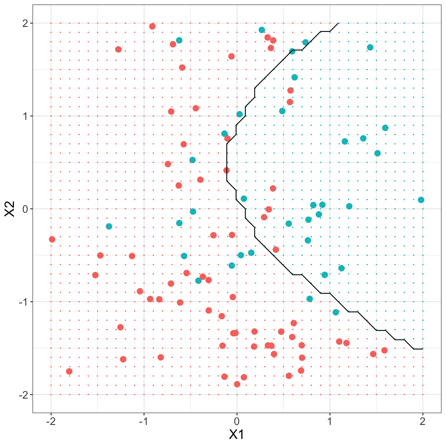
The following plot shows simulated binary data plotted in 2D predictor space, where color corresponds to label. Large dots denote the observations, black line is Bayes decision boundary.

Need for models
Bayes classifier is “gold standard”
In practice, we cannot compute \(p_{ij}(x_{i}) = \textbf{Pr}(y_{i} = j | X = x_{i})\) because we do not know these true probabilities (i.e. we don’t know the true conditional distribution of \(y\) given \(x\))
Instead, we need to estimate the \(p_{ij}(x_{i})\)
Different statistical learning models define different methods to estimate these \(p_{ij}(x_{i})\)!
Once we have an estimate of these conditional class probabilities, the “way” of classifying is the same no matter the model:
- For observation \(i\), predict label \(j^*\) if \(p_{ij^*}(x_{i}) = \max_{j}\{p_{ij}(x_{i})\}\)
Logistic regression
Focus on binary response!
Logistic regression
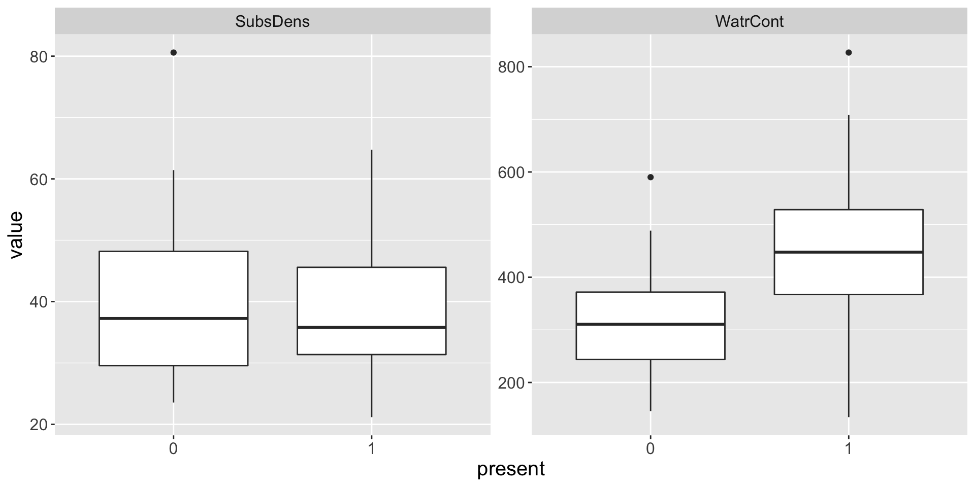
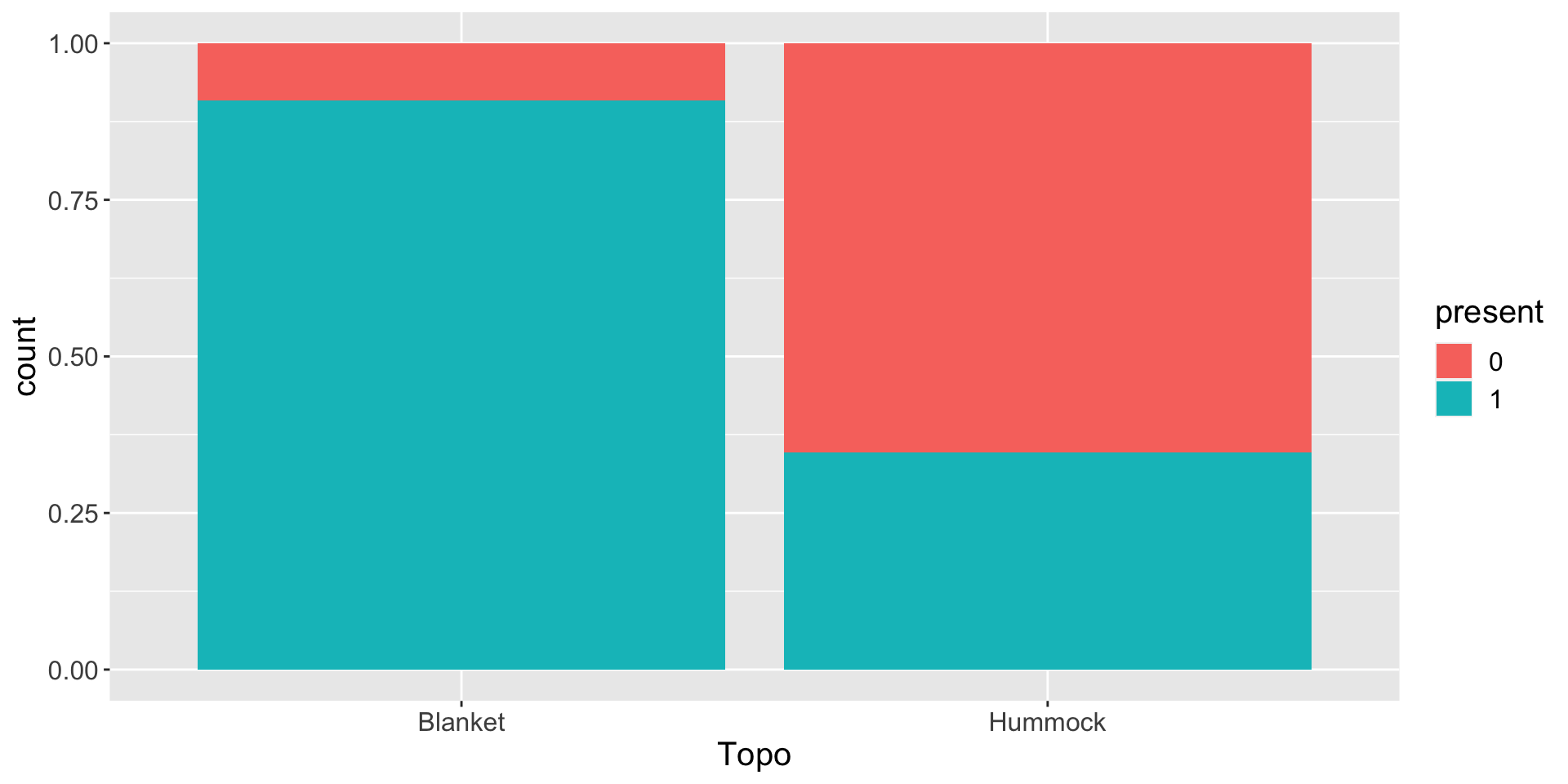
The observed zero abundances in the mite data were difficult to work with. I consider transforming the abundance to a binary response present as follows:


Logistic regression
Fitting a logistic regression:

Logistic regression model
Assume first that we have a single predictor \(X\)
Let \(p({x}) = \text{Pr}(Y = 1 | {X} = {x})\)
- For binary response \((J = 2)\), we shorthand the conditional class probability to always be in terms of a “success” class
Need to somehow restrict \(0 \leq p(x) \leq 1\)
Logistic regression uses logistic function: \[p({x}) = \frac{e^{\beta_{0} + \beta_{1}x}}{1 + e^{\beta_{0} + \beta_{1}x}}\]
Odds and Log-odds
Rearranging this equation yields the odds: \[ \frac{\text{Pr(success)}}{\text{Pr(failure)}} = \frac{p(x)}{1 - p(x)} = e^{\beta_{0} + \beta_{1}x}\]
Furthermore, we can obtain the log-odds: \[\log\left(\frac{p(x)}{1 - p(x)}\right) = \log(e^{\beta_{0} + \beta_{1}x}) = \beta_{0} + \beta_{1}x\]
- When using \(\log()\), we refer to natural logarithm function \(\ln()\)
Interpretation of coefficients
\[\log\left(\frac{p(x)}{1 - p(x)}\right) = \log(e^{\beta_{0} + \beta_{1}x}) = \beta_{0} + \beta_{1}x\]
Interpretation of \(\beta_{1}\): for every one-unit increase in \(x\), we expect an average change of \(\beta_{1}\) in the log-odds (or average multiple of \(e^{\beta_{1}}\) in the odds)
\(\beta_{1}\) does not correspond to the change in \(p(x)\) associated with one-unit increase in \(X\) (i.e., not a linear relationship between \(x\) and \(p(x)\))
If \(\beta_{1} > 0\), then increasing \(x\) is associated with increasing \(p(x)\)
Example
For the mite data, let “success” be when
present = 1; i.e. \(p(x) = \text{Pr}(\text{present} = 1 | X = x)\)I fit the following logistic regression model: \[\log\left(\frac{p(x)}{1-p(x)}\right) = \beta_{0} + \beta_{1} \text{WatrCont}\]
Example (cont.)
Call:
glm(formula = present ~ WatrCont, family = "binomial", data = presence_dat)

Deviance Residuals:
    Min       1Q   Median       3Q      Max
-2.3429  -0.9402   0.4965   0.7911   1.7595

Coefficients:
             Estimate Std. Error z value Pr(>|z|)
(Intercept) -2.481539   1.011855  -2.452  0.01419 *
WatrCont     0.008743   0.002695   3.244  0.00118 **
---
Signif. codes:  0 '***' 0.001 '**' 0.01 '*' 0.05 '.' 0.1 ' ' 1

(Dispersion parameter for binomial family taken to be 1)

    Null deviance: 85.521  on 69  degrees of freedom
Residual deviance: 70.796  on 68  degrees of freedom
AIC: 74.796

Number of Fisher Scoring iterations: 5
Discuss:
What is the interpretation of \(\hat{\beta}_{1} =\) 0.0087?
Is increasing
WatrContassociated with an increasing or decreasing probability of the presence of these mites?
Remarks
Easily extends to \(p\) predictor case: let \(\mathbf{x} = (x_{1}, x_{2}, \ldots, x_{p})\). Then \[\log\left(\frac{p(\mathbf{x})}{1-p(\mathbf{x})}\right) =\beta_{0} + \beta_{1}x_{1} + \ldots \beta_{p} x_{p}\]
Why called logistic “regression” if used for classification task?
- The log-odds is a real-valued quantity that is modeled as a linear function of \(X\)
Obtaining probability
We can interpret the coefficients, but remember the original goal: predict a label (success/failure) for an observation based on its predictors
That is, we want \(p(x)\), not \(\log\left(\frac{p(x)}{1-p(x)}\right)\)
- Let’s simply re-arrange the log-odds formula!
We might ask: what is the estimated probability of presence of mites for a location where
WatrCont = 350?
\[ \begin{align*} &\hat{p}(x) = \frac{e^{\hat{\beta}_{0} + \hat{\beta}_{1}x}}{1 + e^{\hat{\beta}_{0} + \hat{\beta}_{1}x}} \\ &\hat{p}(x = 350) = \frac{e^{-2.4815 + 0.0087 \times 350}}{1+e^{-2.4815 + 0.0087 \times 350}} = 0.637262 \end{align*} \]
- Discuss: based on this model, would you classify an observation with
WatrCont = 350to have mites or not? - Live code!