Regression Trees
Part 2: Pruning
3/16/23
Housekeeping
Lab 03 due tonight
No TA office hours tonight
Lab 04 posted later this afternoon or tomorrow (due Friday after break)
Enjoy your spring break!
Pruning
This next section is a bit technical, but bear with me!
Possible issue
The process of building regression trees may produce good predictions on the training set, but is likely to overfit the data. Why?
A smaller tree with fewer splits/regions might lead to lower variance and better interpretation, at the cost of a little bias
Tree pruning
A better strategy is to grow a very large tree \(T_{0}\), and then prune it back in order to obtain a smaller subtree
Idea: remove sections that are non-critical
Cost complexity pruning or weakest link pruning: consider a sequence of trees indexed by a nonnegative tuning parameter \(\alpha\). For each value of \(\alpha\), there is a subtree \(T \subset T_{0}\) such that \[\left(\sum_{m=1}^{|T|} \sum_{i: x_{i} \in R_{m}} (y_{i} - \hat{y}_{R_{m}})^2 \right)+ \alpha |T|\] is as small as possible.
Cost complexity pruning (cont.)
\[\left(\sum_{m=1}^{|T|} \sum_{i: x_{i} \in R_{m}} (y_{i} - \hat{y}_{R_{m}})^2 \right)+ \alpha |T|\]
\(|T|\) = number of terminal nodes of tree \(T\)
\(R_{m}\) is the rectangle corresponding to the \(m\)-th terminal node
\(\alpha\) controls trade-off between subtree’s complexity and fit to the training data
What is the resultant tree \(T\) when \(\alpha = 0\)?
What happens as \(\alpha\) increases?
Note: for every value of \(\alpha\), we have a different fitted tree \(\rightarrow\) need to choose a best \(\alpha\)
Select an optimal \(\alpha^{*}\) using cross-validation, then return to full data set and obtain the subtree corresponding to \(\alpha^{*}\)
Algorithm for building tree
Suppose I just want to build a “best” regression tree to my data, but I’m not interesting in comparing the performance of my regression tree to a different model.
Using recursive binary splitting to grow a large tree on the data
Apply cost complexity pruning to the large tree in order to obtain a sequence of best trees as a function of \(\alpha\)
Use \(k\)-fold CV to choose \(\alpha\): divide data into \(K\) folds. For each \(k = 1,\ldots, K\):
Repeat Steps 1 and 2 on all but the \(k\)-th fold
Evaluate RMSE on the data in held-out \(k\)-th fold, as a function of \(\alpha\). Average the result for each \(\alpha\)
Choose \(\alpha^{*}\) that minimizes the average error. Return/choose the subtree from Step 2 that corresponds to \(\alpha^{*}\) as your “best” tree!
Algorithm for building tree (comparisons)
If instead I also want to compare my “best” regression tree against a different model, I also need some train/test data to compare the two models
Split data into train and validation sets
Using recursive binary splitting to grow a large tree on the training data
Apply cost complexity pruning to the large tree in order to obtain a sequence of best trees as a function of \(\alpha\)
Use \(k\)-fold CV to choose \(\alpha\): divide training data into \(K\) folds. For each \(k = 1,\ldots, K\):
Repeat Steps 1 and 2 on all but the \(k\)-th fold
Evaluate RMSE on the data in held-out \(k\)-th fold, as a function of \(\alpha\). Average the result for each \(\alpha\)
Choose \(\alpha^{*}\) that minimizes the average error. Return the subtree from Step 2 that corresponds to \(\alpha^{*}\) as “best” tree, and use that tree for predictions on the test data.
- Caution! Note that we have two forms of validation/testing going on here!
Mite data: entire process
Let’s suppose I want to obtain the best regression tree for this mite data, and I want to use the tree to compare to other models
- split data into 80/20 train and validation set
- Use all predictors to build the large tree on the train set
- Perform minimal cost-complexity pruning, to get a sequence of possible/candidate best trees as a function of \(\alpha\)
- Perform 5-fold CV on the training data
- Select \(\alpha^*\)
- For each \(\alpha\), there is an associated CV-error estimate when fitting on the training data (this is the one I care about for choosing one tree). I will choose \(\alpha\) with smallest CV RMSE.
- Prune back the tree from Step 1 according to \(\alpha^*\), and use it to predict for test data
Mite data: entire process (cont.)

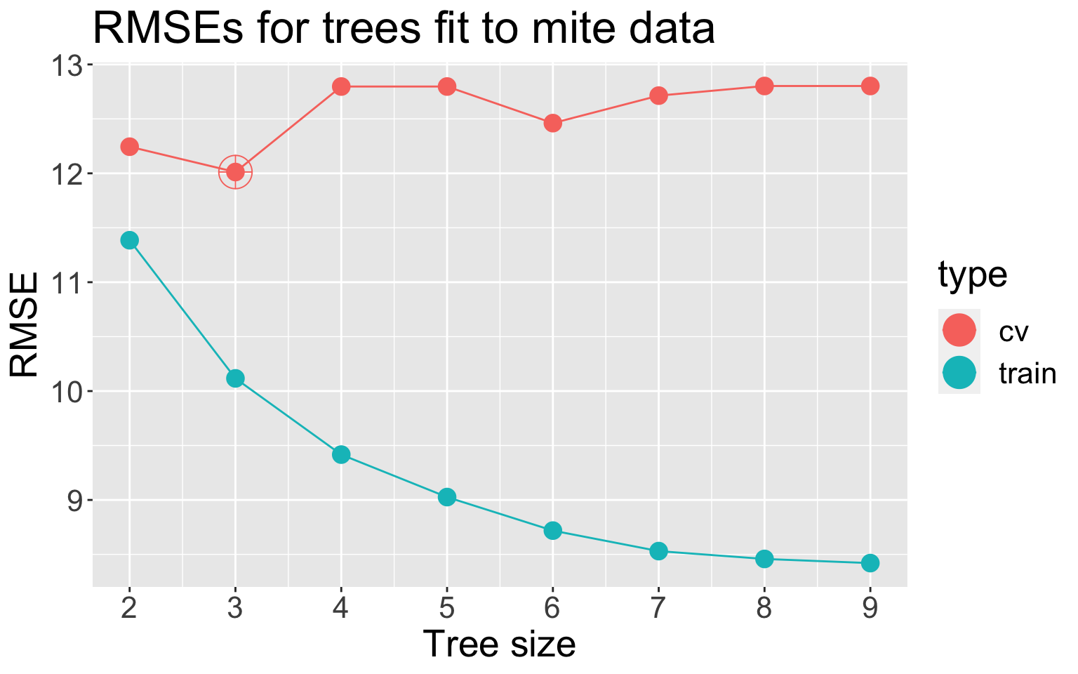
k-fold CV with k = 5. Best CV RMSE (red) at 3 leaves , so this would be our “best” tree
Note: while the CV error is computed as a function of \(\alpha\), we often display as a function of \(|T|\), the number of leaves
Live code
Pruning in R: thankfully much of this is automated!
Summary
Trees vs linear models
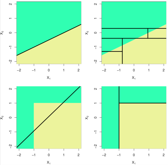
Trees vs. linear models: which is better? Depends on the true relationships between the response and the predictors

Pros and cons
Advantages:
Easy to explain, and may more closely mirror human decision-making than other approaches we’ve seen
Can be displayed graphically and interpreted by non-expert
Can easily handle qualitative predictors without the need to encode or create dummy variables
Making predictions is fast: no calculations needed!
Disadvantages:
Lower levels of predictive accuracy compared to some other approaches
Can be non-robust (high variance)
However, we may see that aggregating many trees can improve predictive performance!