KNN Regression (cont.)

3/7/23

Housekeeping

• KNN implementations: due last night to Canvas (please submit your PDF if you haven’t already)

• Will grade Lab 02: Moneyball today, and hopefully the KNN implementations tomorrow

• Another small KNN regression deliverable due this Thursday 03/09 11:59pm.

K-nearest neighbors: other considerations

Algorithm (recap)

• Choose a positive integer \(K\), and have your data split into a train set and test set

• For a given test observation with predictor \(x_{0}\):

  • Identify the \(K\) points in the train data that are closest (in predictor space) to \(x_{0}\). Call this set of neighbors \(\mathcal{N}_{0}\).

  • Predict \(\hat{y}_{0}\) to be the average of the responses in the neighbor set, i.e. \[\hat{y}_{0} = \frac{1}{K} \sum_{i \in \mathcal{N}_{0}} y_{i}\]

Standardizing predictors

Mite data: preparation

• The following code divides my data into train and test sets.

• Make sure you understand what each line of code is doing! If you don’t, please ask!

set.seed(6)
n <- nrow(mite_dat)
test_ids <- sample(1:n, 2)
train_x <- mite_dat[-test_ids, c("SubsDens", "WatrCont")]
train_y <-  mite_dat$abundance[-test_ids]
test_x <- mite_dat[test_ids,  c("SubsDens", "WatrCont")]
test_y <-  mite_dat$abundance[test_ids]
head(train_x)

  SubsDens WatrCont
1    39.18   350.15
2    54.99   434.81
3    46.07   371.72
4    48.19   360.50
5    23.55   204.13
6    57.32   311.55

Mite data: KNN results

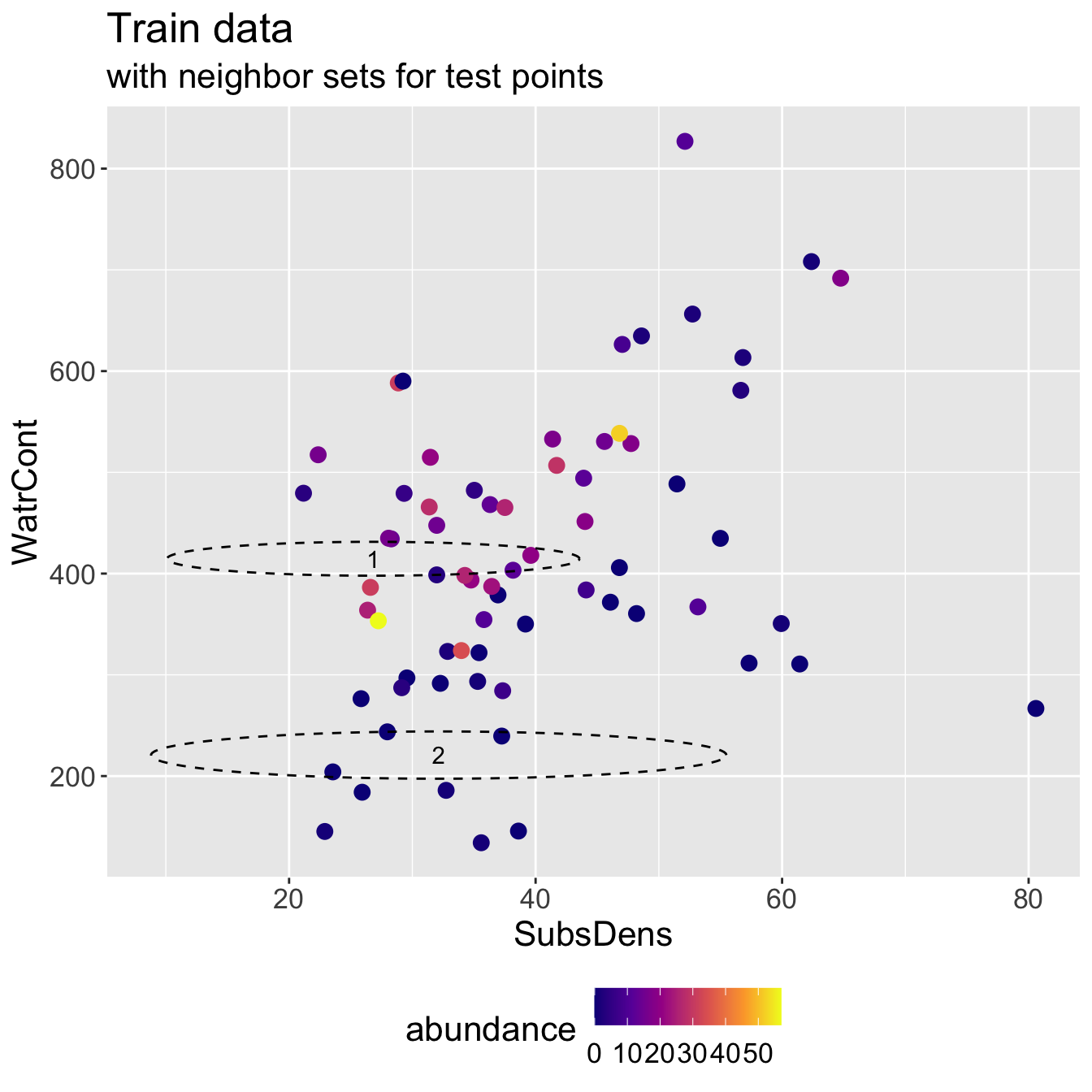
• Running KNN with \(K = 3\) and using Euclidean distance, I identify the following neighbor sets for each test point:

• Predicted abundance \(\hat{y}\) and true abundance \(y\) for both test points, for a test RMSE of 9.428.

# A tibble: 2 × 3
  test_pt y_hat y_true
    <int> <dbl>  <int>
1       1  11.7     25
2       2   0        0

• Discuss: it seems like we did poorly for the first test observation. Does its neighbor set “make sense”?

Standardizing predictors

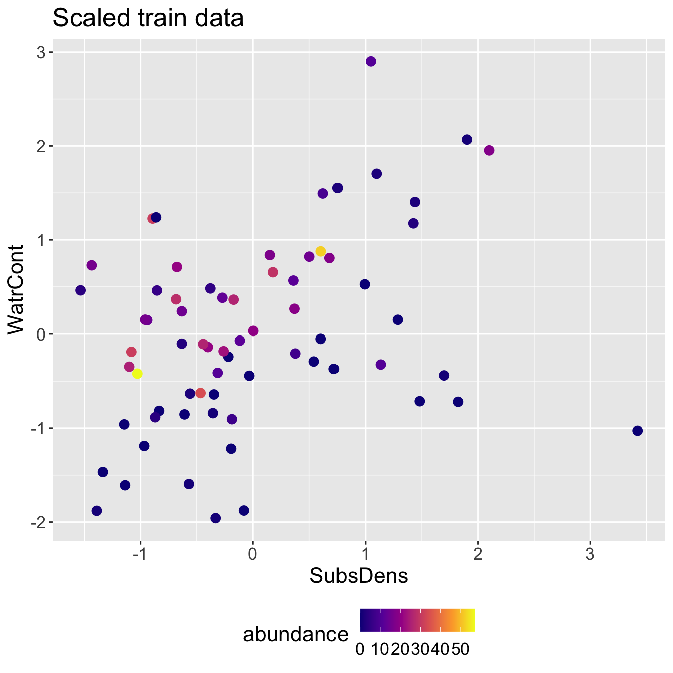
We will standardize our predictors, meaning that each predictor \(X_{j}\) will be transformed to have mean 0 and standard deviation 1:

\[X_{j}^{\text{std}} = \frac{X_{j} - \bar{X_{j}}}{\sigma_{X_{j}}},\]

where \(X_{j}\) is the vector of the \(j\)-th predictor, \(\bar{X}_{j}\) is the average of \(X_{j}\), and \(\sigma_{X_{j}}\) is its standard deviation.

scale(train_x$SubsDens)

              [,1]
 [1,] -0.032638509
 [2,]  1.286001417
 [3,]  0.542024937
 [4,]  0.718844459
 [5,] -1.336265457
 [6,]  1.480336080
 [7,] -0.218632629
 [8,]  3.421180550
 [9,]  1.823132417
[10,] -0.332064020
[11,]  0.602910905
[12,] -0.967613434
[13,] -0.193610999
[14,]  1.698024265
[15,] -0.347076999
[16,] -0.834998793
[17,] -1.145267011
[18,]  0.377716231
[19,] -0.080179607
[20,] -1.137760522
[21,] -0.569769510
[22,] -0.633157640
[23,] -0.608970064
[24,] -0.356251597
[25,]  0.992414286
[26,] -1.390478989
[27,] -0.313714825
[28,] -0.559760858
[29,] -0.116877998
[30,]  0.361035144
[31,] -0.186938564
[32,] -0.261169401
[33,]  1.134203525
[34,] -0.870029076
[35,]  0.003225828
[36,] -0.401290531
[37,]  0.681312014
[38,]  2.100038461
[39,] -0.442993249
[40,] -0.272012107
[41,] -1.081878880
[42,]  1.424454439
[43,]  1.902367580
[44,]  0.603744959
[45,]  0.370209741
[46,] -0.466346771
[47,]  0.178377241
[48,] -1.101062130
[49,] -0.940923695
[50,] -0.171925585
[51,] -0.893382597
[52,]  0.501990329
[53,] -0.633157640
[54,]  0.150853448
[55,]  1.438633362
[56,] -1.028499402
[57,]  1.097505134
[58,] -0.684034956
[59,]  0.622094155
[60,]  0.752206633
[61,] -0.378771064
[62,] -0.959272891
[63,] -1.534770392
[64,] -0.676528467
[65,]  1.046627818
[66,] -0.861688532
[67,] -0.854182043
[68,] -1.435517924
attr(,"scaled:center")
[1] 39.57132
attr(,"scaled:scale")
[1] 11.98963

# confirming we have mean 0 and sd 1
scaled_SubsDens <- scale(train_x$SubsDens)
mean(scaled_SubsDens)

[1] -4.865389e-16

sd(scaled_SubsDens)

[1] 1

Standardizing multiple variables

train_x_scaled <- train_x %>%
  mutate_if(is.numeric, scale)
head(train_x_scaled)

     SubsDens   WatrCont
1 -0.03263851 -0.4434260
2  1.28600142  0.1503860
3  0.54202494 -0.2921323
4  0.71884446 -0.3708303
5 -1.33626546 -1.4676219
6  1.48033608 -0.7141694

train_x_scaled <- train_x
train_x_scaled$SubsDens <- scale(train_x$SubsDens)
train_x_scaled$WatrCont <- scale(train_x$WatrCont)
head(train_x_scaled)

     SubsDens   WatrCont
1 -0.03263851 -0.4434260
2  1.28600142  0.1503860
3  0.54202494 -0.2921323
4  0.71884446 -0.3708303
5 -1.33626546 -1.4676219
6  1.48033608 -0.7141694

Standardizing the test data

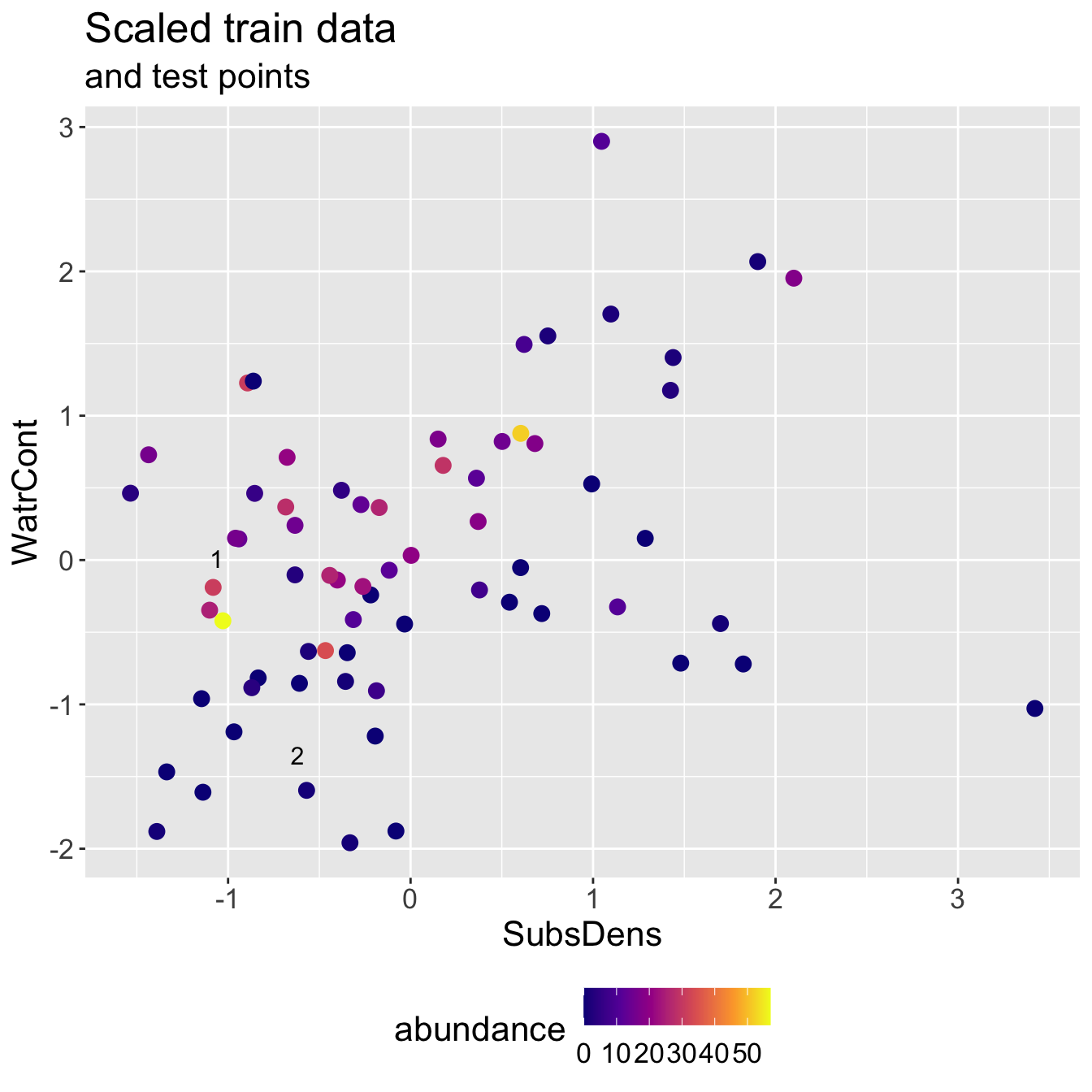
• We should use the same statistics from the training data to scale the test data

  • i.e. to standardize the \(j\)-th predictor of the test data, we should use the mean and standard deviation of the \(j\)-th predictor from the training data

• Discuss: why not scale the predictors first, and then split into train/test sets?

# note: I am not providing you the code for how I scaled my test observations!
test_x_scaled

     SubsDens     WatrCont
53 -1.0626956  0.008982148
10 -0.6198128 -1.351188146

• Important:
  • I do not scale the response variable
  • I scale after splitting into train/test

Scaled mite data

Scaled mite data: KNN results

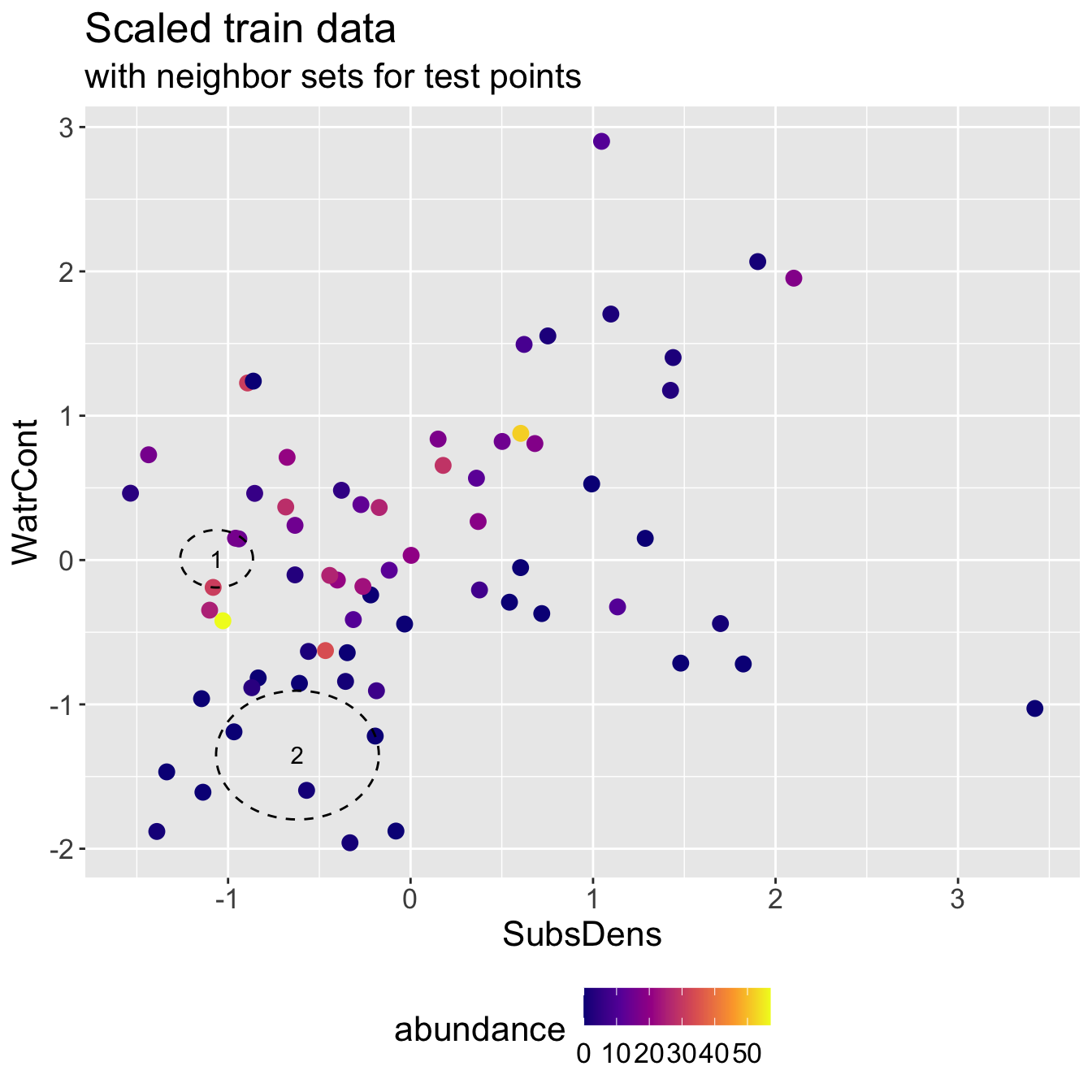
• Predicted abundance \(\hat{y}\) and true abundance \(y\) for both test points, for a test RMSE of 3.308.

# A tibble: 2 × 3
  test_pt  y_hat y_true
    <int>  <dbl>  <int>
1       1 20.3       25
2       2  0.333      0

• Note how this RMSE compares to when we fit on original scale!

  • Even though we do slightly worse predicting test point 2, we improve a lot on test point 1

Categorical predictors

Why are categorical predictors a problem?

• Suppose we want to include the categorical predictors into our predictions:

• Topo \(\in \{ \text{Blanket, Hummock}\}\)

• Shrub \(\in \{\text{None, Few, Many} \}\)

• Substrate \(\in \{\text{Sphagn1, Spaghn2, Sphagn3, Sphagn4, Litter, Barepeat, Interface}\}\)

• Discuss: how would you define “distance” or “closeness” between two observations based on:

  • Topo

  • Shrub

• We will create new quantitative variables to represent categorical variables

Integer encoding

• The predictor Shrub is ordinal

  • i.e. there is a natural ordering (None < Few < Many) to the \(L = 3\) categories

• The ordering should be reflected in the new quantitative variable

• Integer encoding: convert each label (category/level) into an integer value, where:

  • “Lowest” level gets assigned 0
  • Second lowest level gets assigned 1
  • …
  • “Highest” level gets assigned \(L-1\)

• Live code

Mite data: integer encoding

   Shrub Shrub_encode
68  None            0
39   Few            1
1    Few            1
34  Many            2
43   Few            1

• Now I can calculate distances using Shrub_encode!

One-hot encoding

• Question: why wouldn’t I want to use integer encoding for a non-ordinal variable such as Substrate?

• One-hot encoding: map each level of the variable to a new binary 0/1 variable, where

  • 0 represents the absence of the category
  • 1 represents the presence of the category

• These are called “dummy variables”; will have \(L\) new variables

• Live code

Mite data: one-hot encoding

One-hot encoding of the Topo variable:

      Topo Topo_hummock Topo_blanket
68 Blanket            0            1
39 Blanket            0            1
1  Hummock            1            0
34 Blanket            0            1
43 Blanket            0            1

Mite data: one-hot encoding (cont.)

One-hot encoding of the Substrate variable:

# A tibble: 8 × 8
  Substrate Sub_Sphagn1 Sub_Litter Sub_Interface Sub_S…¹ Sub_S…² Sub_S…³ Sub_B…⁴
  <fct>           <dbl>      <dbl>         <dbl>   <dbl>   <dbl>   <dbl>   <dbl>
1 Sphagn2             0          0             0       0       0       1       0
2 Interface           0          0             1       0       0       0       0
3 Barepeat            0          0             0       0       0       0       1
4 Sphagn1             1          0             0       0       0       0       0
5 Sphagn1             1          0             0       0       0       0       0
6 Interface           0          0             1       0       0       0       0
7 Sphagn2             0          0             0       0       0       1       0
8 Interface           0          0             1       0       0       0       0
# … with abbreviated variable names ¹​Sub_Sphagn3, ²​Sub_Sphagn4, ³​Sub_Sphagn2,
#   ⁴​Sub_Barepeat

Mite data: final data set

So, our final set of predictors X that we could use in KNN regression for the response variable abundance would be:

# A tibble: 70 × 12
   SubsDens WatrCont Shrub_encode Topo_hummock Topo_blanket Sub_Sphagn1
      <dbl>    <dbl>        <dbl>        <dbl>        <dbl>       <dbl>
 1     46.8     406.            1            1            0           1
 2     37.3     284.            2            0            1           0
 3     29.2     590.            0            0            1           1
 4     28.9     588.            0            0            1           1
 5     46.8     539.            1            0            1           0
 6     26.8     415.            0            0            1           0
 7     47.0     626.            0            0            1           0
 8     48.6     635.            0            0            1           0
 9     56.6     581             1            0            1           0
10     27.2     353.            0            0            1           1
   Sub_Litter Sub_Interface Sub_Sphagn3 Sub_Sphagn4 Sub_Sphagn2 Sub_Barepeat
        <dbl>         <dbl>       <dbl>       <dbl>       <dbl>        <dbl>
 1          0             0           0           0           0            0
 2          0             1           0           0           0            0
 3          0             0           0           0           0            0
 4          0             0           0           0           0            0
 5          0             1           0           0           0            0
 6          0             1           0           0           0            0
 7          0             1           0           0           0            0
 8          0             1           0           0           0            0
 9          0             1           0           0           0            0
10          0             0           0           0           0            0
# … with 60 more rows

• Discuss: what are some potential issues with one-hot encoding?

Summary

• Key point: when computing distances, you should consider standardizing your predictors if they are on very different scales

• To calculate distances between categorical variables, we need to encode them somehow

• Questions:

  • Should we standardize our new encoded variables?

  • Does anything need to change about your current KNN implementation to address standardizing variables and/or accommodating categorical predictors?