KNN Regression

2/28/23

Housekeeping

• Lab 02 due Thursday to Canvas at 11:59pm

• Office hours today from 3-4pm

• TA: Doug Rosin

  • Office hours Sundays 7-9pm upstairs

K-nearest neighbors

(Warning: there will be a lot of \(K\)’s in this course!)

K-nearest neighbors

• K-nearest neighbors (KNN) is a nonparametric supervised learning method

• Intuitive and simple

• Relies on the assumption: observations with similar predictors will have similar responses

• Works for both regression and classification (we will start with regression)

Algorithm (in words)

• Choose a positive integer \(K\), and have your data split into a train set and test set

• For a given test observation with predictor \(x_{0}\):

  • Identify the \(K\) points in the train data that are closest (in predictor space) to \(x_{0}\). Call this set of neighbors \(\mathcal{N}_{0}\).

  • Predict \(\hat{y}_{0}\) to be the average of the responses in the neighbor set, i.e. \[\hat{y}_{0} = \frac{1}{K} \sum_{i \in \mathcal{N}_{0}} y_{i}\]

Example

• On the next slide, you will see plot with a bunch of colored points

• Each point is plotted in predictor space \((x1, x2)\), and is colored according to the value of its response \(y\)

• I have a new point (\(\color{blue}{*}\)) and its covariates/predictors, but I need to make a prediction for its response

Example (cont.)

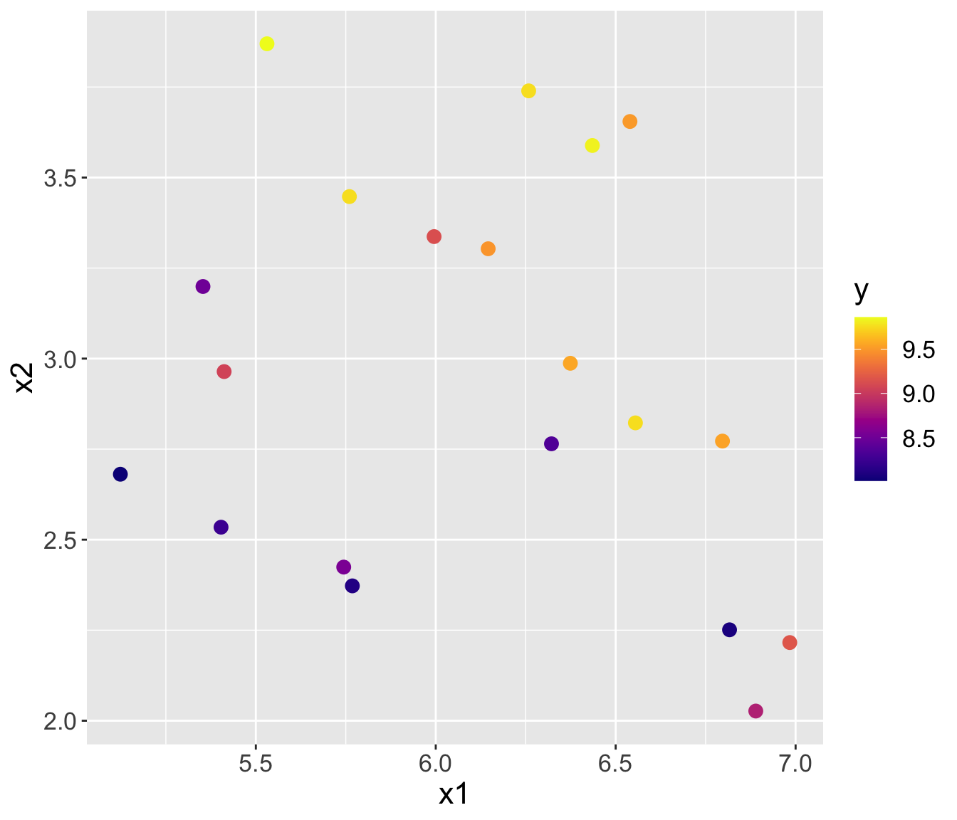
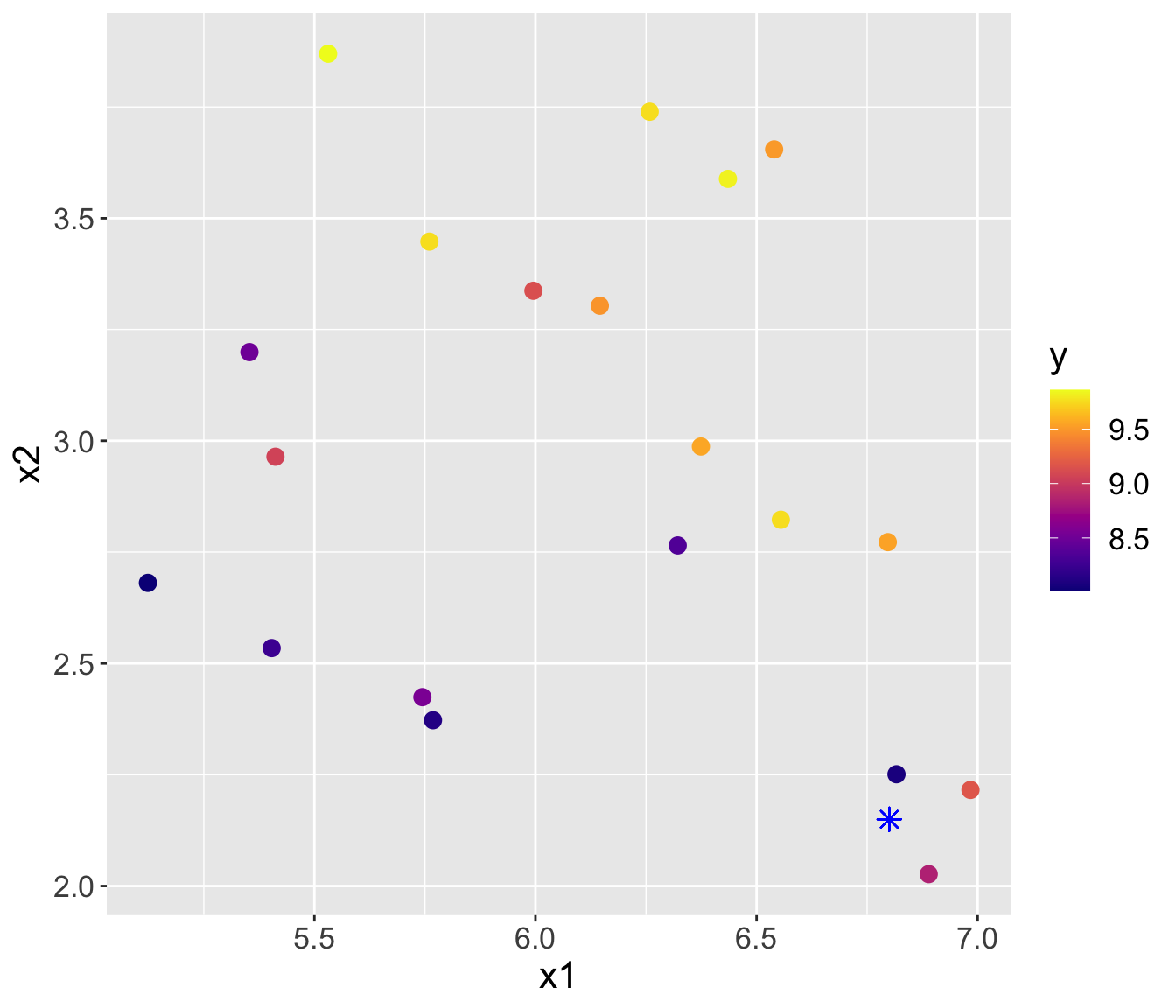
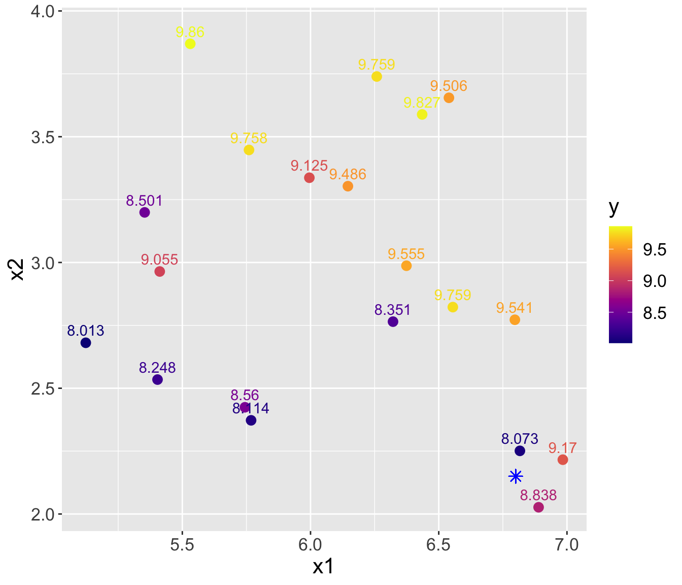
• Using \(K= 3\), predicted \(\hat{y}_{0} = \frac{1}{3}(8.073 + 8.838 + 9.17) = 8.694\)

• Using \(K= 4\), predicted \(\hat{y}_{0} = \frac{1}{4}(8.073 + 8.838 + 9.17 + 9.541) = 8.906\)

Considerations

1. How do we determine who the neighbors \(\mathcal{N}_{0}\) should be? On the previous slide, it may have seemed intuitive.

   • i.e. how do we quantify “closeness”?

2. Which \(K\) should we use?

Consideration 1: Closeness

• We will quantify closeness using distance metrics

Euclidean distance

• One of the most common ways to measure distance between points is with Euclidean distance

• On a number line (one-dimension), the distance between two points \(a\) and \(b\) is simply the absolute value of their difference

  • Let \(d(a,b)\) denote the Euclidean distance between \(a\) and $b$. Then in 1-D, \(d(a,b) = |a-b|\).

• In 2-D (think lon-lat coordinate system), the two points are \(\mathbf{a} = (a_{1}, a_{2})\) and \(\mathbf{b} = (b_{1}, b_{2})\) with Euclidean distance \[d(\mathbf{a}, \mathbf{b}) = \sqrt{(a_{1} - b_{1}) ^2 + (a_{2} - b_{2})^2}\]

• Important: the “two-dimensions” refers to the number of coordinates in each point, not the fact that we are calculating a distance between two points

Euclidean distance (cont.)

• Generalizing to \(p\) dimensions: if \(\mathbf{a} = (a_{1}, a_{2}, \ldots, a_{p})\) and \(\mathbf{b} = (b_{1}, b_{2}, \ldots, b_{p})\), then \[d(\mathbf{a}, \mathbf{b}) = \sqrt{(a_{1} - b_{1}) ^2 + (a_{2} - b_{2})^2 + \ldots (a_{p} - b_{p})^2} = \sqrt{\sum_{j=1}^{p}(a_{j} - b_{j})^2}\]

• E.g. let \(\mathbf{a} = (1, 0, 3)\) and \(\mathbf{b} = (-1, 2, 2)\). What is \(d(\mathbf{a}, \mathbf{b})\)?

Euclidean distance

• Another common distance metric is Manhattan distance

  • Named after the grid-system of Manhattan’s roads

• The Manhattan distance between two points \(\mathbf{a}\) and \(\mathbf{b}\) in \(p\)-dimensions is \[d_{m}(\mathbf{a}, \mathbf{b}) = |a_{1} - b_{1}| + |a_{2} - b_{2}| + \ldots +|a_{p} - b_{p}| = \sum_{j=1}^{p} |a_{j} - b_{j}|\]

• E.g. let \(\mathbf{a} = (1, 0, 3)\) and \(\mathbf{b} = (-1, 2, 2)\). What is \(d_{m}(\mathbf{a}, \mathbf{b})\)?

Distance in KNN

• We want to find the closest neighbor(s) in the train set to a given test point \(\mathbf{x}_{0}\), such that we can make a prediction \(\hat{y}_{0}\).

• Important: what would the points \(\mathbf{a}\) and \(\mathbf{b}\) be in KNN?

Practice

  X1 X2 X3 y
1  1  1 -1 0
2  2  0  0 2
3 -1  1  0 4
4  0  1  0 6

• Suppose I have the above data, and I want to predict for a new test point x0 with X1 = 0, X2 = 0, X3 = 0.

• Calculate the distance between x0 and each of the observed data points using:

  • Euclidean distance

  • Manhattan distance

Consideration 2: K

How much does K matter?

• It can matter a lot!

• As we saw previously, you will get different predicted \(\hat{y}_{0}\) for different choices of \(K\) in KNN regression

• Discuss:

  • What does \(K=1\) mean? Do you think \(K = 1\) is a good choice?

  • It is better to choose a small \(K\) or big \(K\)?

Example: mite data

Mite data: preparation

• The following code divides my data into train and test sets.

• Make sure you understand what each line of code is doing! If you don’t, please ask!

set.seed(6)
n <- nrow(mite_dat)
test_ids <- sample(1:n, 2)
train_x <- mite_dat[-test_ids, c("SubsDens", "WatrCont")]
train_y <-  mite_dat$abundance[-test_ids]
test_x <- mite_dat[test_ids,  c("SubsDens", "WatrCont")]
test_y <-  mite_dat$abundance[test_ids]
head(train_x)

  SubsDens WatrCont
1    39.18   350.15
2    54.99   434.81
3    46.07   371.72
4    48.19   360.50
5    23.55   204.13
6    57.32   311.55

Mite data: KNN

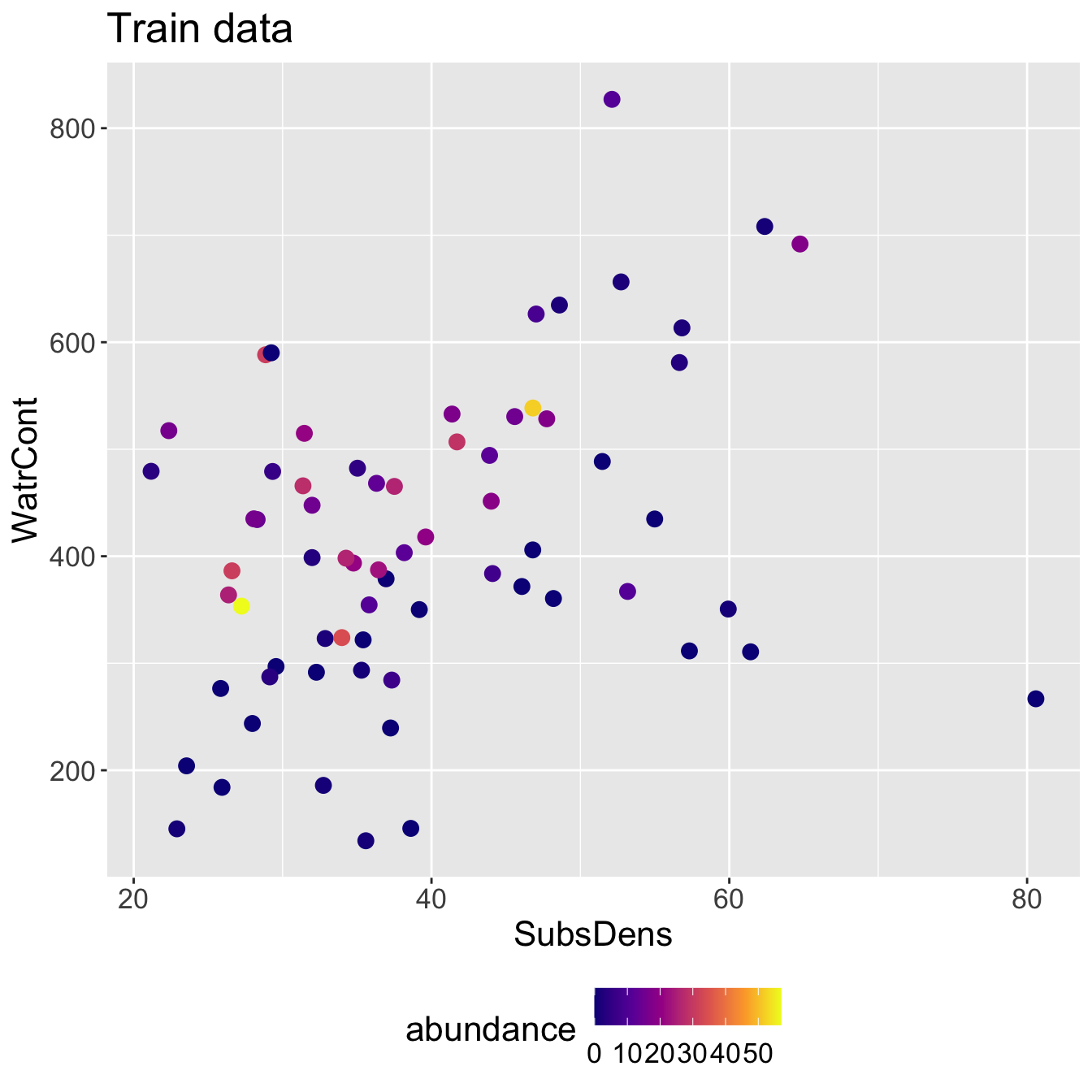
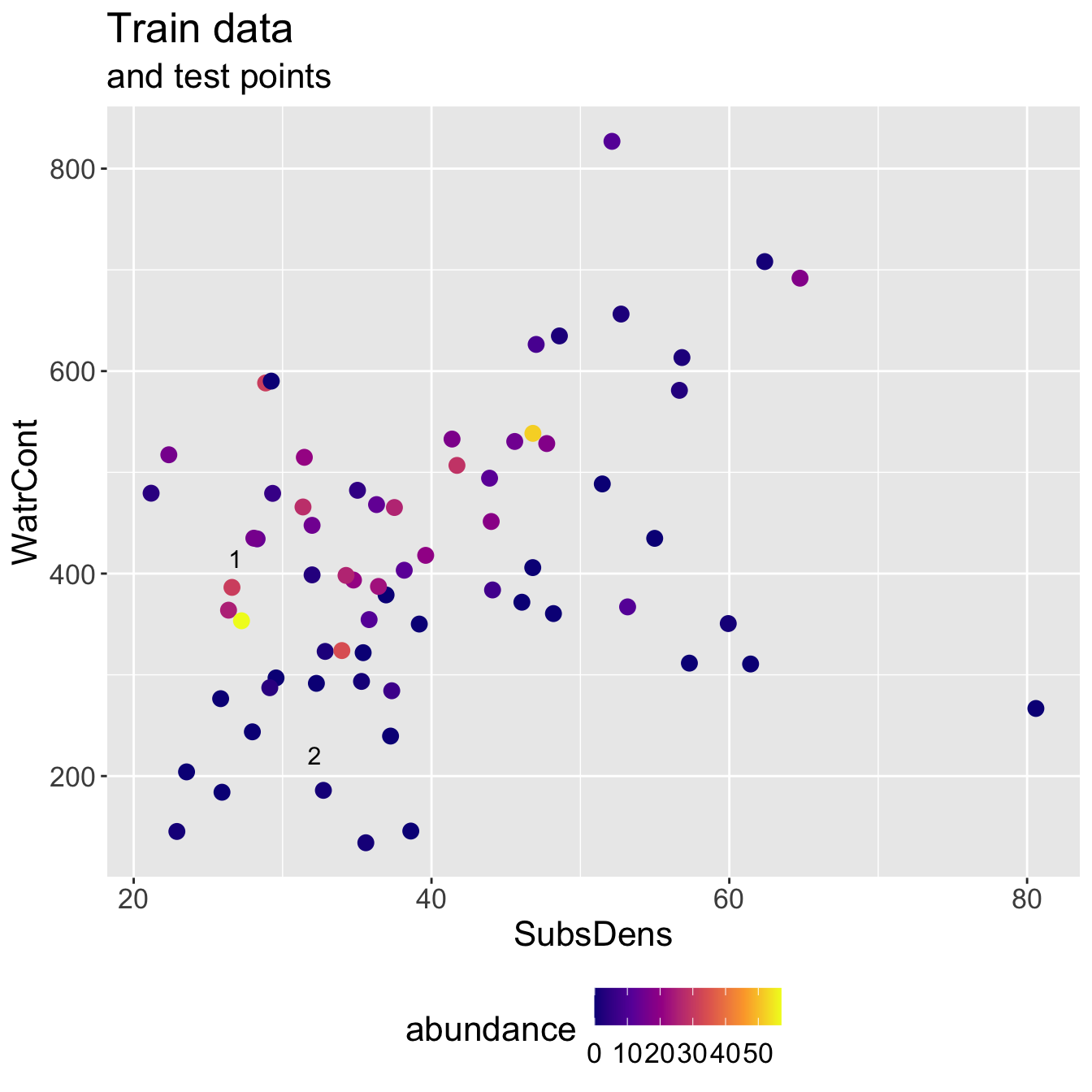
Mite data: KNN results

• Running KNN with \(K = 3\) and using Euclidean distance, I identify the following neighbor sets for each test point:

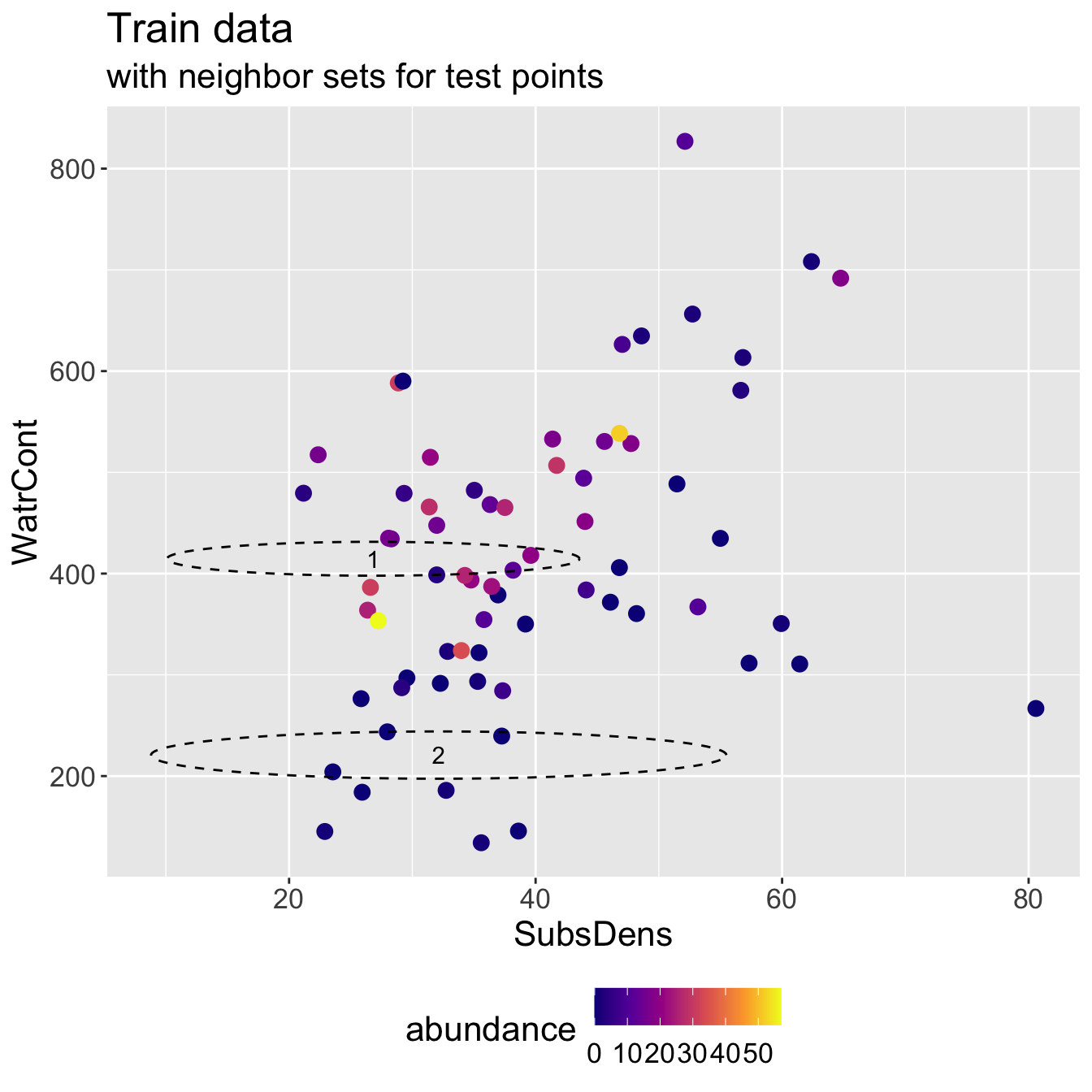
• Predicted abundance \(\hat{y}\) and true abundance \(y\) for both test points, for a test RMSE of 9.428.

# A tibble: 2 × 3
  test_pt y_hat y_true
    <int> <dbl>  <int>
1       1  11.7     25
2       2   0        0

• Discuss: it seems like we did poorly for the first test observation. Does its neighbor set “make sense”?

Standardizing predictors

We will standardize our predictors, meaning that each predictor \(X_{j}\) will be transformed to have mean 0 and standard deviation 1:

\[X_{j}^{\text{std}} = \frac{X_{j} - \bar{X_{j}}}{\sigma_{X_{j}}},\]

where \(X_{j}\) is the vector of the \(j\)-th predictor, \(\bar{X}_{j}\) is the average of \(X_{j}\), and \(\sigma_{X_{j}}\) is its standard deviation.

scale(train_x$SubsDens)

              [,1]
 [1,] -0.032638509
 [2,]  1.286001417
 [3,]  0.542024937
 [4,]  0.718844459
 [5,] -1.336265457
 [6,]  1.480336080
 [7,] -0.218632629
 [8,]  3.421180550
 [9,]  1.823132417
[10,] -0.332064020
[11,]  0.602910905
[12,] -0.967613434
[13,] -0.193610999
[14,]  1.698024265
[15,] -0.347076999
[16,] -0.834998793
[17,] -1.145267011
[18,]  0.377716231
[19,] -0.080179607
[20,] -1.137760522
[21,] -0.569769510
[22,] -0.633157640
[23,] -0.608970064
[24,] -0.356251597
[25,]  0.992414286
[26,] -1.390478989
[27,] -0.313714825
[28,] -0.559760858
[29,] -0.116877998
[30,]  0.361035144
[31,] -0.186938564
[32,] -0.261169401
[33,]  1.134203525
[34,] -0.870029076
[35,]  0.003225828
[36,] -0.401290531
[37,]  0.681312014
[38,]  2.100038461
[39,] -0.442993249
[40,] -0.272012107
[41,] -1.081878880
[42,]  1.424454439
[43,]  1.902367580
[44,]  0.603744959
[45,]  0.370209741
[46,] -0.466346771
[47,]  0.178377241
[48,] -1.101062130
[49,] -0.940923695
[50,] -0.171925585
[51,] -0.893382597
[52,]  0.501990329
[53,] -0.633157640
[54,]  0.150853448
[55,]  1.438633362
[56,] -1.028499402
[57,]  1.097505134
[58,] -0.684034956
[59,]  0.622094155
[60,]  0.752206633
[61,] -0.378771064
[62,] -0.959272891
[63,] -1.534770392
[64,] -0.676528467
[65,]  1.046627818
[66,] -0.861688532
[67,] -0.854182043
[68,] -1.435517924
attr(,"scaled:center")
[1] 39.57132
attr(,"scaled:scale")
[1] 11.98963

# confirming we have mean 0 and sd 1
scaled_SubsDens <- scale(train_x$SubsDens)
mean(scaled_SubsDens)

[1] -4.865389e-16

sd(scaled_SubsDens)

[1] 1

Standardizing multiple variables

train_x_scaled <- train_x %>%
  mutate_if(is.numeric, scale)
head(train_x_scaled)

     SubsDens   WatrCont
1 -0.03263851 -0.4434260
2  1.28600142  0.1503860
3  0.54202494 -0.2921323
4  0.71884446 -0.3708303
5 -1.33626546 -1.4676219
6  1.48033608 -0.7141694

train_x_scaled <- train_x
train_x_scaled$SubsDens <- scale(train_x$SubsDens)
train_x_scaled$WatrCont <- scale(train_x$WatrCont)
head(train_x_scaled)

     SubsDens   WatrCont
1 -0.03263851 -0.4434260
2  1.28600142  0.1503860
3  0.54202494 -0.2921323
4  0.71884446 -0.3708303
5 -1.33626546 -1.4676219
6  1.48033608 -0.7141694

Standardizing the test data

• We should use the same statistics from the training data to scale the test data

  • i.e. to standardize the \(j\)-th predictor of the test data, we should use the mean and standard deviation of the \(j\)-th predictor from the training data

• Discuss: why not scale the predictors first, and then split into train/test sets?

# note: I am not providing you the code for how I scaled my test observations!
test_x_scaled

     SubsDens     WatrCont
53 -1.0626956  0.008982148
10 -0.6198128 -1.351188146

• Important:
  • I do not scale the response variable
  • I scale after splitting into train/test

Scaled mite data

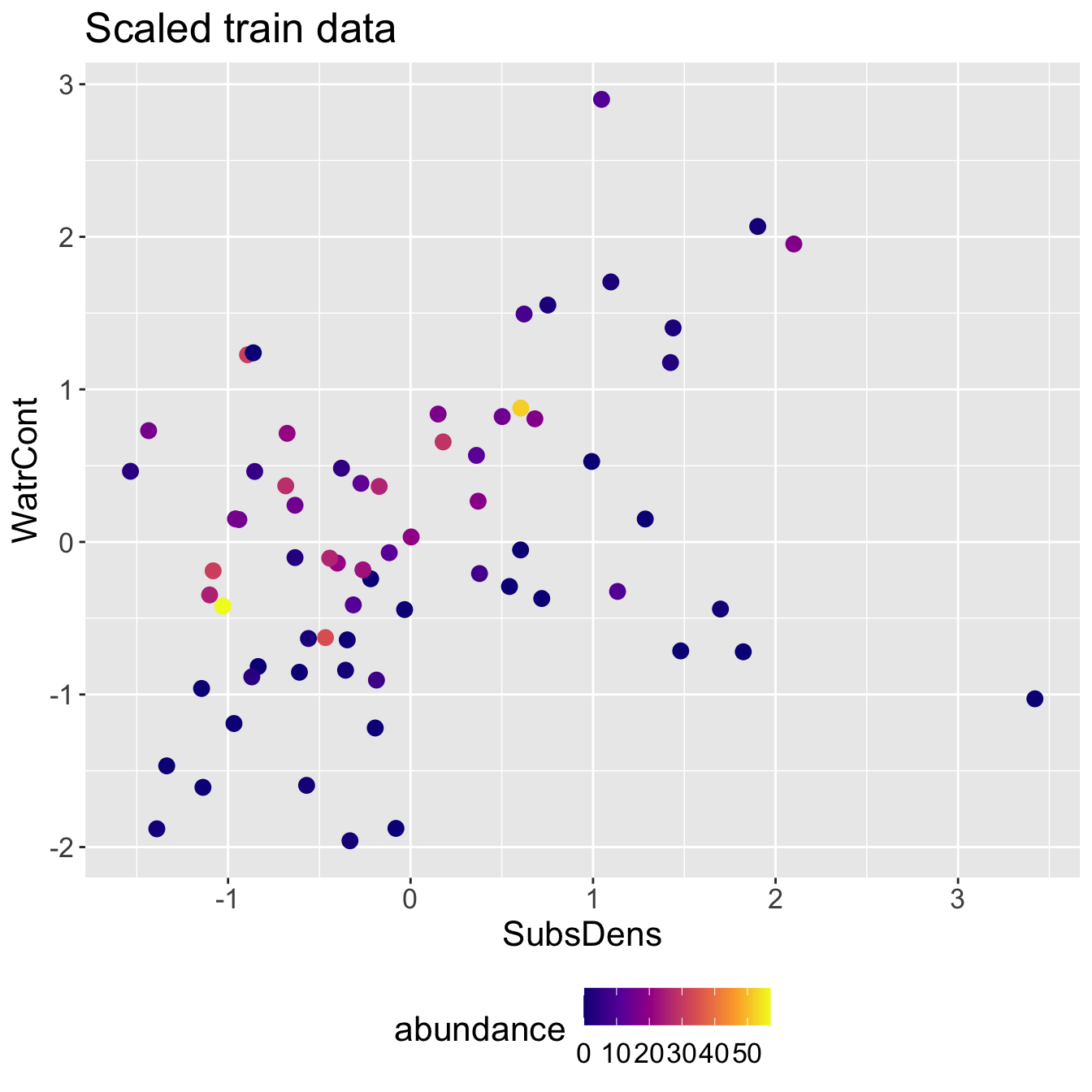
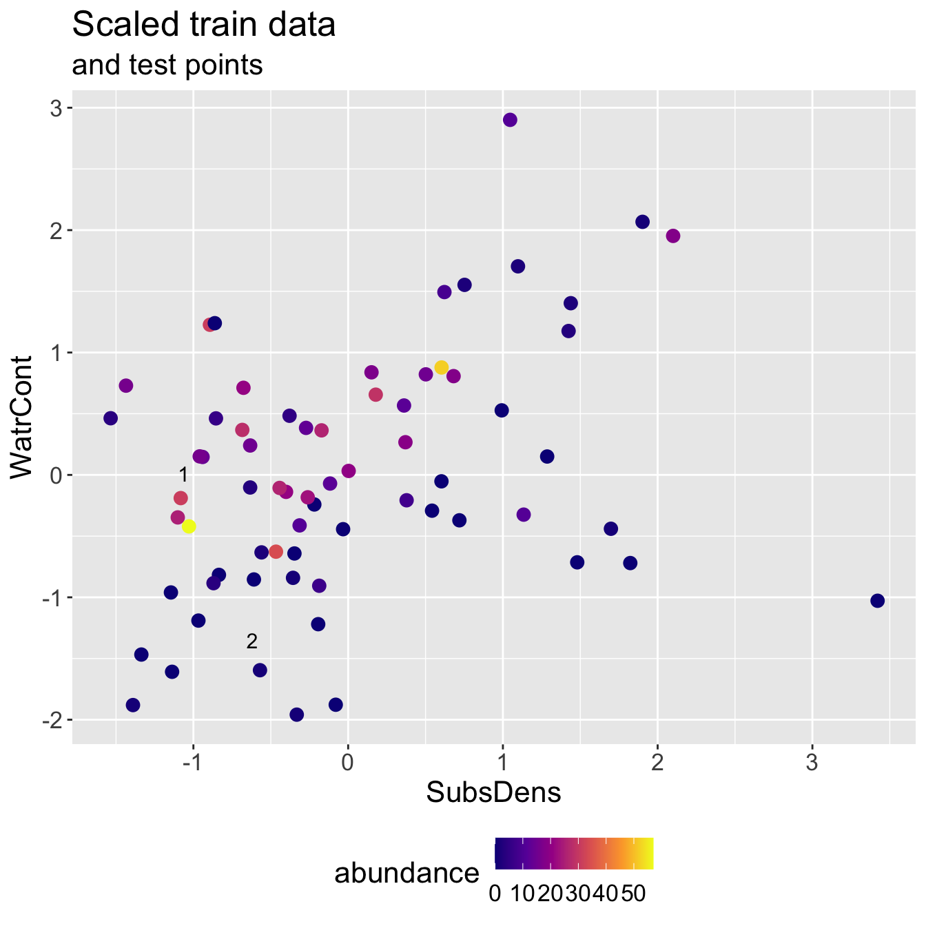
Scaled mite data: KNN results

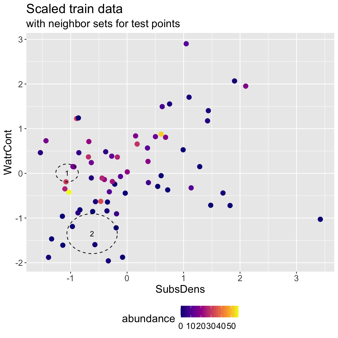
• Predicted abundance \(\hat{y}\) and true abundance \(y\) for both test points, for a test RMSE of 3.308.

# A tibble: 2 × 3
  test_pt  y_hat y_true
    <int>  <dbl>  <int>
1       1 20.3       25
2       2  0.333      0

• Note how this RMSE compares to when we fit on original scale!

  • Even though we do slightly worse predicting test point 2, we improve a lot on test point 1

Summary

• Looking forward:

  • You will implement KNN this week in small groups!

  • We will learn later on in the semester how we might pick \(K\)

  • What about categorical predictors?