Linear Regression

2/23/23

Housekeeping

Lab 01 due tonight to Canvas at 11:59pm
Lab 02 assigned tomorrow (and has to do with baseball)

Linear regression

A simple, widely used approach in supervised learning
Assumes that the dependence of \(Y\) on the predictors \(X_{1}, \ldots, X_{p}\) is linear

Possible questions of interest

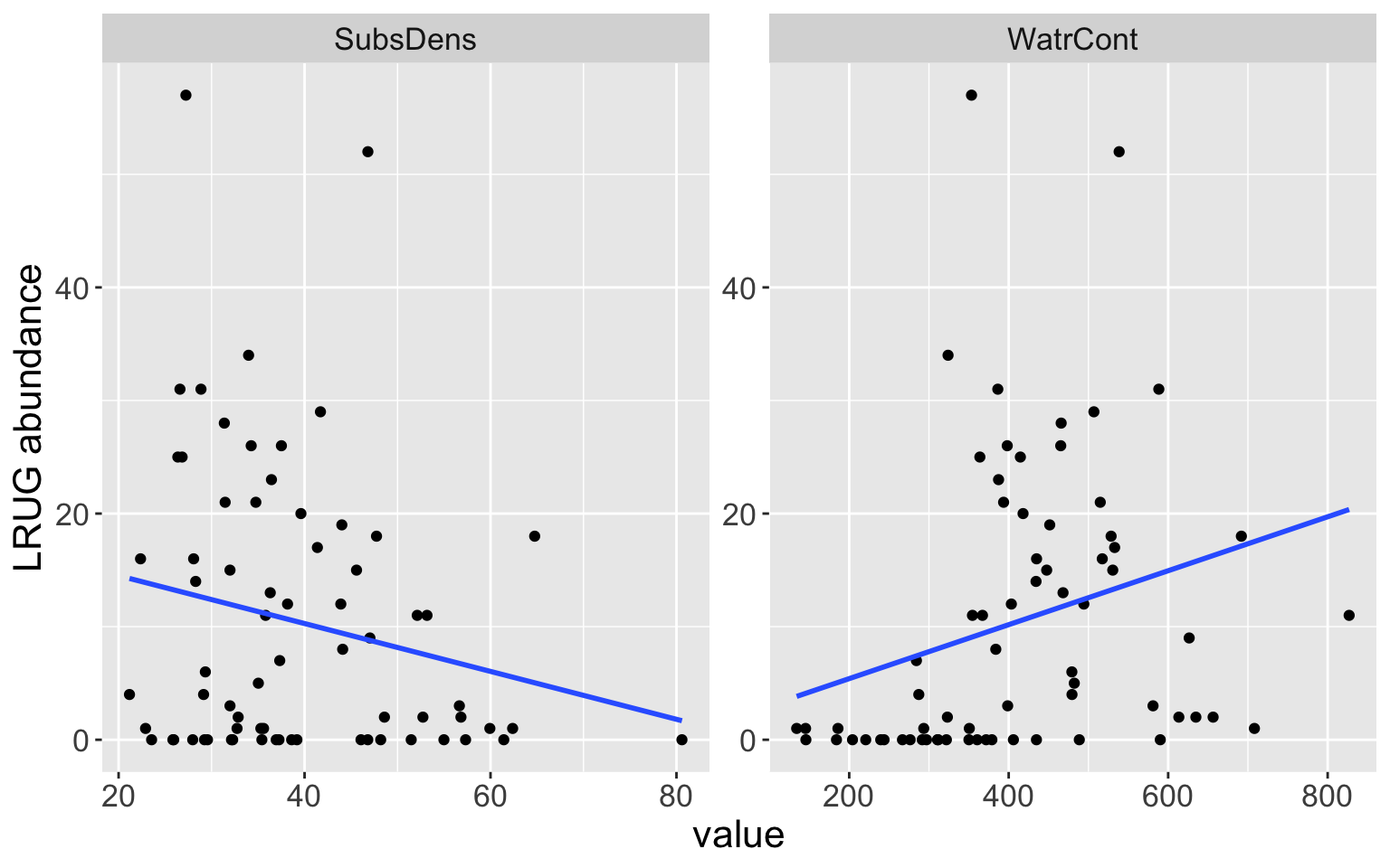
Is there a relationship between the abundance of LRUG mites and substrate density or water content in the soil where they are found?
- If so, how are strong are these relationships?
Is the relationship linear?
How accurately can we predict the abundance of these mites?

Simple Linear Regression

Simple linear regression

Simple linear regression (SLR)
- Assumes a linear model for a quantitative response \(Y\) using a single predictor \(X\)
  
  \[Y = \beta_{0} + \beta_{1} X + \epsilon,\]
  
  where \(\beta_{0}, \beta_{1}\) are unknown coefficients (parameters) and \(\epsilon\) is the error
\(\beta_{0}\) is commonly referred to as the intercept, and \(\beta_{1}\) is the slope
For example: abundance = \(\beta_{0}\) + \(\beta_{1}\) watercont + \(\epsilon\)

Parameter estimation

Assuming \(n\) observations, we have data of the form \((x_{1}, y_{1}), (x_{2}, y_{2}), \ldots, (x_{n}, y_{n})\)
An SLR model says \[\begin{align*} y_{i} &= \beta_{0} + \beta_{1}x_{i}+ \epsilon\\ &\approx \beta_{0} + \beta_{1}x_{i}\ , \qquad \text{ for all } i = 1,\ldots, n \end{align*}\]
- In this model, \(f(x_{i}) = \beta_{0} + \beta_{1} x_{i}\)
- Notice that the relationship between \(x_{i}\) and \(y_{i}\) is the same for all \(i\)
In practice, \(\beta_{0}\) and \(\beta_{1}\) are unknown, so we must estimate them
Goal: obtain (good) estimates \(\hat{\beta}_{0}\) and \(\hat{\beta}_{1}\) that are as close to the true values as possible, such that \(y_{i} \approx \hat{\beta}_{0} + \hat{\beta}_{1} x_{i}\)
- How? Minimize the least squares criterion

Least squares

Let \(\hat{y}_{i} = \hat{\beta}_{0} + \hat{\beta}_{1}x_{i}\) be predicted response for \(i\)-th observation with predictor \(x_{i}\)
The \(i\)-th residual \(e_{i}\) is defined as \[e_{i} = y_{i} - \hat{y}_{i}\]
Define residual sum of squares (RSS) as \[\text{RSS} = e_{1}^{2} + e_{2}^{2} + \ldots + e_{n}^{2} = \sum_{i=1}^{n} e_{i}^2\]

Estimation by least squares

\[\text{RSS} = \sum_{i=1}^{n} e_{i}^2 = \sum_{i=1}^{n} (y_{i} - \hat{y}_{i})^2 = \sum_{i=1}^{n} (y_{i} - (\hat{\beta}_{0} + \hat{\beta}_{1}x_{i}))^2\]

Least squares approach selects the pair \((\hat{\beta}_{0}, \hat{\beta}_{1})\) that minimize the RSS. Can be shown that the minimizing values are: \[\begin{align*} \hat{\beta}_{1} &= \frac{\sum_{i=1}^{n}(x_{i} - \bar{x})(y_{i} - \bar{y})}{\sum_{i=1}^{n}(x_{i} - \bar{x})^2}\\ \hat{\beta}_{0} &= \bar{y} - \hat{\beta}_{1} \bar{x} \end{align*}\]

where \(\bar{y} = \frac{1}{n}\sum_{i=1}^{n}y_{i}\) and \(\bar{x} = \frac{1}{n}\sum_{i=1}^{n}x_{i}\)

Mite data

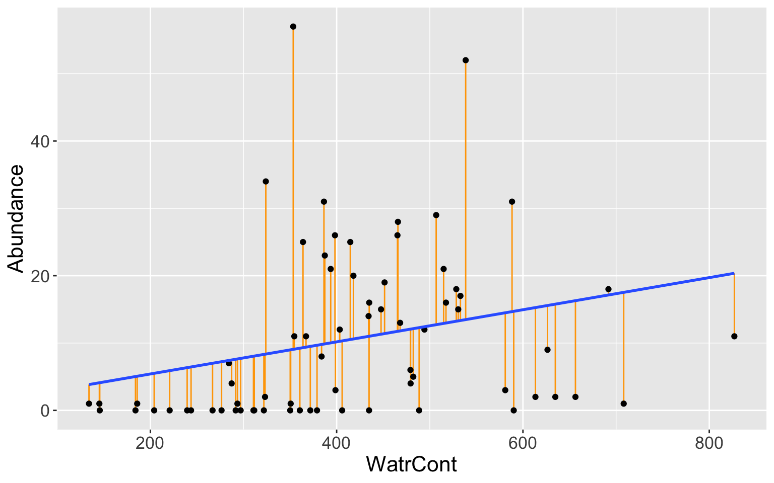
Least squares fit for abundance regressed on WaterCont, with residuals in orange.

m1 <- lm(abundance ~ WatrCont, data = mite_dat)

Let’s interpret this plot! Do you see anything strange or any patterns?

Interpreting Coefficients and Estimates

\[Y = \beta_{0} + \beta_{1} X + \epsilon\]

\(\beta_{0}\) is the expected value of \(Y\) when \(X = 0\)
\(\beta_{1}\) is the average increase in \(Y\) for one-unit increase in \(X\)
\(\epsilon\) is error
This equation is the population regression line
When using the least squares estimates for the coefficients, \(\hat{Y} = \hat{\beta}_{0} + \hat{\beta}_{1} X\) is the least squares line

Interpreting Coefficients and Estimates (cont.)

summary(m1)


Call:
lm(formula = abundance ~ WatrCont, data = mite_dat)

Residuals:
    Min      1Q  Median      3Q     Max 
-16.525  -8.033  -4.088   4.493  47.937 

Coefficients:
            Estimate Std. Error t value Pr(>|t|)  
(Intercept)  0.63410    4.51171   0.141   0.8886  
WatrCont     0.02385    0.01039   2.296   0.0248 *
---
Signif. codes:  0 '***' 0.001 '**' 0.01 '*' 0.05 '.' 0.1 ' ' 1

Residual standard error: 12.29 on 68 degrees of freedom
Multiple R-squared:  0.07194,   Adjusted R-squared:  0.05829 
F-statistic: 5.271 on 1 and 68 DF,  p-value: 0.02477

\[\widehat{\text{LRUG}} = 0.634 + 0.024 \text{WatrCont}\]

How do I interpret \(\hat{\beta}_{0}\) and \(\hat{\beta}_{1}\) for this specific example?
Note: the estimates \(\hat{\beta}_{0}\) and \(\hat{\beta}_{1}\) will depend on the observed data! If I took a different sample of LRUG mites, I would probably have different estimated values.
- Isn’t that problematic? Can we asses how accurate are our estimates \(\hat{\beta}_{0}\) and \(\hat{\beta}_{1}\)?

Assessing Accuracy of Coefficient Estimates

Standard error (SE) of an estimator reflects how it varies under repeated sampling.
For simple linear regression: \[\text{SE}(\hat{\beta}_{0}) = \sigma^2 \left[ \frac{1}{n} + \frac{\bar{x}^2}{\sum_{i=1}^{n}(x_{i} - \bar{x})^2}\right] \qquad \text{SE}(\hat{\beta}_{1}) = \frac{\sigma^2}{\sum_{i=1}^{n}(x_{i} - \bar{x})^2}\]

where \(\sigma^2 = \text{Var}(\epsilon)\)
Typically \(\sigma^2\) is not known, but can be estimated from the data.
Estimate \(\hat{\sigma}\) is residual standard error (RSE), given by: \[\hat{\sigma}= \text{RSE} = \sqrt{\frac{1}{n-2}\text{RSS}}\]
We use this estimate to calculate \(\text{SE}(\hat{\beta}_{0})\) and \(\text{SE}(\hat{\beta}_{1})\)

Hypothesis Testing

Hypothesis testing is a method of statistical inference to determine whether the data at hand sufficiently support a particular hypothesis
- Helps test the results of an experiment or survey to see if you have meaningful results
- Helps draw conclusions about a population parameter
Standard errors can be used to perform hypothesis tests on the coefficients

Hypothesis Testing

Notion of “null” versus “alternate” hypothesis
- Null hypothesis \(H_{0}\): there is no relationship between \(X\) and \(Y\)
- Alternative hypothesis \(H_{A}\): there is some relationship between \(X\) and \(Y\)
Mathematically, corresponds to testing \[H_{0}: \beta_{1} = 0 \quad \text{ vs. } \quad H_{A}: \beta_{1} \neq 0\]

because if \(H_{0}\) true, then the model reduces to \(Y = \beta_{0} + \epsilon\) so there is no relationship
To test this null hypothesis, want to determine if \(\hat{\beta}_{1}\) is sufficiently far from zero
- How much is ‘sufficiently far’? Depends on \(\text{SE}(\hat{\beta}_{1})\).

p-value

With lots of hand-waving: can calculate a p-value, which is a probability that we observed the data we did, given that \(H_{0}\) is true. If the p-value is small, the observed data don’t seem to support \(H_{0}\)
- Compare \(p\)-value to a pre-determined rejection level \(\alpha\) (often 0.05).
- If \(p\)-value \(< \alpha\), reject \(H_{0}\). Otherwise, fail to reject \(H_{0}\).

summary(m1)


Call:
lm(formula = abundance ~ WatrCont, data = mite_dat)

Residuals:
    Min      1Q  Median      3Q     Max 
-16.525  -8.033  -4.088   4.493  47.937 

Coefficients:
            Estimate Std. Error t value Pr(>|t|)  
(Intercept)  0.63410    4.51171   0.141   0.8886  
WatrCont     0.02385    0.01039   2.296   0.0248 *
---
Signif. codes:  0 '***' 0.001 '**' 0.01 '*' 0.05 '.' 0.1 ' ' 1

Residual standard error: 12.29 on 68 degrees of freedom
Multiple R-squared:  0.07194,   Adjusted R-squared:  0.05829 
F-statistic: 5.271 on 1 and 68 DF,  p-value: 0.02477

\(H_{0}: \beta_{1} = 0\) (there is no relationship between LRUG abundance and WatrCont)
- What is the p-value for this hypothesis?
- What is our decision in the mite example?

Why hypothesis testing?

Hypothesis testing can help us determine if there is a relationship between the predictor and the response variable!
- This is the inference part of statistical learning
If there is a relationship, then it makes sense to interpret the strength of the relationship (i.e. interpret the value \(\hat{\beta}_{1}\))

Multiple Linear Regression

Multiple linear regression

In practice, we often have more than one predictor
With \(p\) predictors, the model is \[Y = \beta_{0} + \beta_{1}X_{1} + \beta_{2}X_{2} + \ldots + \beta_{p}X_{p} +\epsilon\]
Interpret \(\beta_{j}\) as the average effect on \(Y\) for a one-unit increase in \(X_{j}\), holding all other predictors fixed/constant

Mite data

Regressing abundance on both WatrCont and SubsDens:

m2 <- lm(abundance ~ WatrCont + SubsDens, data = mite_dat)
summary(m2)


Call:
lm(formula = abundance ~ WatrCont + SubsDens, data = mite_dat)

Residuals:
    Min      1Q  Median      3Q     Max 
-20.192  -8.633  -1.385   6.866  44.245 

Coefficients:
            Estimate Std. Error t value Pr(>|t|)   
(Intercept) 10.30549    5.48833   1.878  0.06477 . 
WatrCont     0.03444    0.01057   3.257  0.00177 **
SubsDens    -0.35682    0.12604  -2.831  0.00612 **
---
Signif. codes:  0 '***' 0.001 '**' 0.01 '*' 0.05 '.' 0.1 ' ' 1

Residual standard error: 11.7 on 67 degrees of freedom
Multiple R-squared:  0.1711,    Adjusted R-squared:  0.1464 
F-statistic: 6.915 on 2 and 67 DF,  p-value: 0.001861

\[\widehat{abundance} = 10.306 + 0.034 \text{WatrCont} -0.357 \text{SubsDens}\]

How do we interpret the estimated coefficients?
How do we interpret the p-values?
- The p-value for \(\beta_{j}\) corresponds to the test of \(H_{0}: \beta_{j} = 0\) and \(\beta_{k} (k \neq j)\) unrestricted

Model assessment

Model fit

How well does our linear regression model “fit” the data it was trained on? How accurate is our model?
Residual standard error (RSE) \[\text{RSE} = \sqrt{\frac{1}{n-p-1} \sum_{i=1}^{n} (y_{i} - \hat{y}_{i})^2},\]

where \(p\) is the number of predictors, and \(i\) indexes the observations used to fit the model
RSE is considered a measure of the lack of fit of the model
- Measured in the units of \(Y\)

Predictions

How well does our linear regression model predict new responses for a given set of covariates?
For example, suppose I want to use our model to predict the abundance of LRUG mites at a new sampling location where the WatrCont is 400 g/L and the SubsDens is 30 g/L
I will plug these values into our fitted model m2:

\[\widehat{abundance} = 10.306 + 0.034 \times 400 -0.357 \times 30 = 13.3747829\]

new_data <- data.frame(WatrCont = 400, SubsDens = 30)
pred_mite <- predict(m2, newdata = new_data)

Okay…great! But should I trust these predictions?

Prediction performance

We could get a better sense of a model’s prediction performance by comparing the predicted responses to the true values
We should always compare prediction performance for “previously unseen” data (i.e. test data)
- The model already “knows” the data used to fit it (i.e. the training data)
Discuss: what are some important criteria for the testing data?

Qualitative predictors

Thus far, we have assumed that all predictors in our linear model are quantitative. In practice, we often have categorical predictors
Our mite data has the following categorical variables: Shrub, Substrate, and Topo
Let’s begin with the simplest case: a categorical predictor with two categories/levels
- e.g. the Topo variable takes on the values “Blanket” or “Hummock” only

2-level qualitative predictor

We will create an indicator or dummy variable as follows: \[\text{TopoBlanket}_{i} = \begin{cases} 1 & \text{ if } \color{blue}{\text{Topo}_{i}} = \text{Blanket} \\ 0 & \text{ if } \color{blue}{\text{Topo}_{i}} = \text{Hummock} \end{cases}\]
Simple linear regression model for LRUG regressed on Topo: \[\text{LRUG}_{i} = \beta_{0} + \beta_{1}\text{TopoBlanket}_{i} + \epsilon_{i} = \begin{cases} \beta_{0} + \epsilon_{i} & \text{ if } \color{blue}{\text{Topo}_{i}} = \text{Blanket} \\ \beta_{0} + \beta_{1} + \epsilon_{i} & \text{ if } \color{blue}{\text{Topo}_{i}} = \text{Hummock} \end{cases}\]
How to interpret?

Mite data

m3 <- lm(abundance ~ Topo, data = mite_dat)
summary(m3)


Call:
lm(formula = abundance ~ Topo, data = mite_dat)

Residuals:
    Min      1Q  Median      3Q     Max 
-15.318  -4.318  -2.154   4.473  41.682 

Coefficients:
            Estimate Std. Error t value Pr(>|t|)    
(Intercept)   15.318      1.658   9.238 1.26e-13 ***
TopoHummock  -13.164      2.721  -4.838 7.85e-06 ***
---
Signif. codes:  0 '***' 0.001 '**' 0.01 '*' 0.05 '.' 0.1 ' ' 1

Residual standard error: 11 on 68 degrees of freedom
Multiple R-squared:  0.2561,    Adjusted R-squared:  0.2452 
F-statistic: 23.41 on 1 and 68 DF,  p-value: 7.851e-06

Fitted model is: \[\widehat{\text{LRUG}} = 15.318 - 13.164 \text{TopoHummock}\]
Interpret!

More than two levels

With more than two levels, we simply create additional dummy variables: \[\begin{align*}\text{Shrub}_{i,Few} &= \begin{cases} 1 & \text{ if } \color{blue}{\text{Shrub}_{i}} = \text{Few} \\ 0 & \text{ if } \color{blue}{\text{Shrub}_{i}} = \text{not Few} \end{cases} \\ \text{Shrub}_{i, Many} &= \begin{cases} 1 & \text{ if } \color{blue}{\text{Shrub}_{i}} = \text{Many} \\ 0 & \text{ if } \color{blue}{\text{Shrub}_{i}} = \text{not Many} \end{cases} \end{align*}\]
Resulting regression model for LRUG with only Shrub as predictor: \[\begin{align*} \text{LRUG}_{i} &= \beta_{0} + \beta_{1} \text{Shrub}_{i, Few} + \beta_{2} \text{Shrub}_{i, Many} + \epsilon_{i}\\ &\approx \begin{cases} \beta_{0} + \beta_{1} & \text{ if } \color{blue}{\text{Shrub}_{i}} = \text{Few} \\ \beta_{0} + \beta_{2} & \text{ if } \color{blue}{\text{Shrub}_{i}} = \text{Many} \\ \beta_{0} & \text{ if } \color{blue}{\text{Shrub}_{i}} = \text{None} \end{cases}\end{align*}\]

m4 <- lm(abundance ~ Shrub, data = mite_dat)
summary(m4)


Call:
lm(formula = abundance ~ Shrub, data = mite_dat)

Residuals:
    Min      1Q  Median      3Q     Max 
-16.895  -8.060  -2.760   6.635  40.105 

Coefficients:
            Estimate Std. Error t value Pr(>|t|)    
(Intercept)   10.923      1.405   7.775 6.12e-11 ***
Shrub.L       -9.288      2.505  -3.707 0.000427 ***
Shrub.Q       -1.460      2.359  -0.619 0.538164    
---
Signif. codes:  0 '***' 0.001 '**' 0.01 '*' 0.05 '.' 0.1 ' ' 1

Residual standard error: 11.64 on 67 degrees of freedom
Multiple R-squared:  0.1791,    Adjusted R-squared:  0.1545 
F-statistic: 7.306 on 2 and 67 DF,  p-value: 0.001348

Remarks

For a given categorical variable, there will always be one fewer dummy variables than levels
- Level with no dummy variable is known as baseline. For model m4 on previous slide, the “None” category was the baseline level
Can have multiple categorical variables in a single model:

m5 <- lm(abundance ~ Topo + Shrub, data = mite_dat)
summary(m5)


Call:
lm(formula = abundance ~ Topo + Shrub, data = mite_dat)

Residuals:
    Min      1Q  Median      3Q     Max 
-16.895  -6.056   0.691   4.756  40.105 

Coefficients:
            Estimate Std. Error t value Pr(>|t|)    
(Intercept)   14.755      1.641   8.993 4.48e-13 ***
TopoHummock  -11.253      2.997  -3.755 0.000369 ***
Shrub.L       -4.832      2.580  -1.873 0.065552 .  
Shrub.Q       -3.128      2.203  -1.420 0.160385    
---
Signif. codes:  0 '***' 0.001 '**' 0.01 '*' 0.05 '.' 0.1 ' ' 1

Residual standard error: 10.65 on 66 degrees of freedom
Multiple R-squared:  0.3236,    Adjusted R-squared:  0.2928 
F-statistic: 10.52 on 3 and 66 DF,  p-value: 9.593e-06

Let’s write out the estimated regression model together
- What does \(\beta_{0}\) represent?
- How do we interpret the coefficients?

Extensions of linear model (optional)

Linear model is restrictive

Linear model is widely used and works quite well, but has several highly restrictive assumptions
- Relationship between \(X\) and \(Y\) is additive
- Relationship between \(X\) and \(Y\) is linear
There are common approaches to loosen these assumptions. We will only discuss the first restriction here. Take a regression class for more!

Interactions

Additive assumption: the association between a predictor \(X_{j}\) and the response \(Y\) does not depend on the value of any other predictors

\[Y = \beta_{0} + \beta_{1} X_{1} + \beta_{2} X_{2} + \epsilon\]

\[Y = \beta_{0} + \beta_{1} X_{1} + \beta_{2} X_{2} + \beta_{3}\color{orange}{X_{1}X_{2}} + \epsilon\]

This third predictor \(\color{orange}{X_{1}X_{2}}\) is known as an interaction term
The total effect of \(X_{1}\) on \(Y\) also depends on the value of \(X_{2}\) through the interaction
In the above equation, \(\beta_{1}\) and \(\beta_{2}\) are called the “main effects” of \(X_{1}\) and \(X_{2}\) respectively

Mite data

Suppose I want to regress LRUG abundance on SubsDens and WatrCont and their interaction:

mod_int <- lm(abundance ~ SubsDens + WatrCont + 
                SubsDens * WatrCont,
              data = mite_dat)
summary(mod_int)


Call:
lm(formula = abundance ~ SubsDens + WatrCont + SubsDens * WatrCont, 
    data = mite_dat)

Residuals:
    Min      1Q  Median      3Q     Max 
-24.012  -7.155  -1.896   5.011  44.539 

Coefficients:
                    Estimate Std. Error t value Pr(>|t|)  
(Intercept)       -1.012e+01  1.369e+01  -0.740   0.4621  
SubsDens           1.323e-01  3.256e-01   0.406   0.6859  
WatrCont           8.667e-02  3.379e-02   2.565   0.0126 *
SubsDens:WatrCont -1.210e-03  7.443e-04  -1.625   0.1088  
---
Signif. codes:  0 '***' 0.001 '**' 0.01 '*' 0.05 '.' 0.1 ' ' 1

Residual standard error: 11.56 on 66 degrees of freedom
Multiple R-squared:  0.203, Adjusted R-squared:  0.1668 
F-statistic: 5.604 on 3 and 66 DF,  p-value: 0.001744

Mite data

Fitted model: \(\widehat{LRUG} = -10.12 + 0.132 \text{SubsDens} + 0.087 \text{WatrCont} -0.001 \text{SubsDens} \times \text{WatrCont}\)
Interpretations?

Estimates suggest that a 1 g/L increase in the \(\color{blue}{\text{WaterCont}}\) of the soil is associated with an increased abundance of (0.087 + -0.001 \(\times \color{blue}{\text{SubsDens}}\)) LRUG mites

Interactions with categorical variable

Can also have interactions involving categorical variables!
In particular, the interaction between a quantitative and a categorical variable has nice interpretation
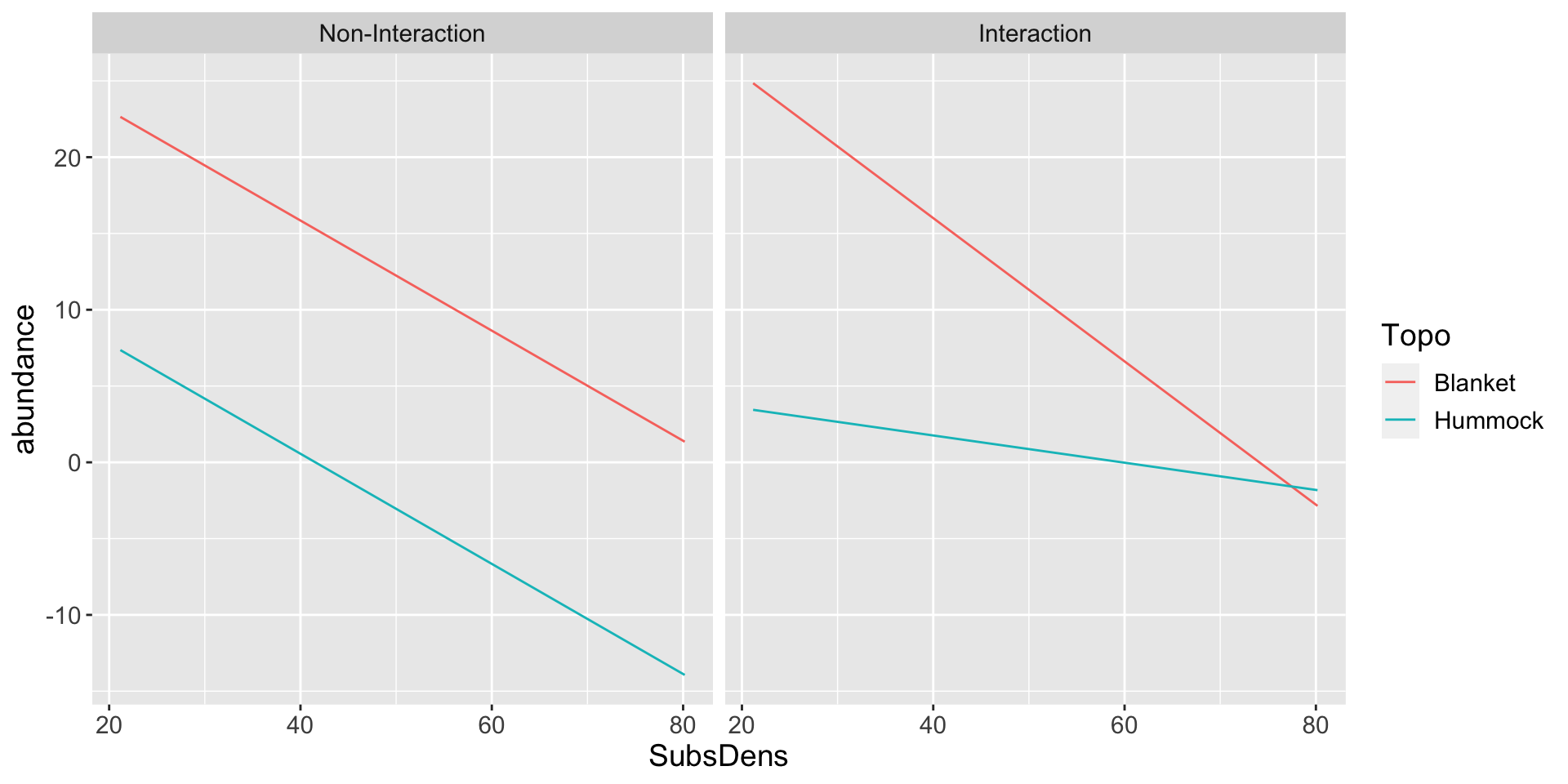
Consider the effects of SubsDens and Topo and their interaction on the abundances: \[\begin{align*} \text{LRUG}_{i} &\approx \beta_{0} + \beta_{1} \text{SubsDens}_{i} + \beta_{2}\text{TopoBlanket}_{i} + \beta_{3} \text{SubsDens}_{i} \times \text{TopoBlanket}_{i} \\ & = \begin{cases} \beta_{0} + \beta_{1}\text{SubsDens}_{i} & \text{ if } \color{blue}{\text{Topo}_{i}} = \text{Blanket} \\ (\beta_{0} + \beta_{2}) + (\beta_{1} + \beta_{3}) \text{SubsDens}_{i} & \text{ if } \color{blue}{\text{Topo}_{i}} = \text{Hummock} \end{cases} \end{align*}\]


Call:
lm(formula = abundance ~ SubsDens + Topo + SubsDens * Topo, data = mite_dat)

Residuals:
    Min      1Q  Median      3Q     Max 
-21.059  -4.764  -1.186   3.229  39.191 

Coefficients:
                     Estimate Std. Error t value Pr(>|t|)    
(Intercept)           34.7881     5.3697   6.479 1.35e-08 ***
SubsDens              -0.4695     0.1242  -3.781 0.000338 ***
TopoHummock          -29.4584     9.0331  -3.261 0.001757 ** 
SubsDens:TopoHummock   0.3803     0.2323   1.637 0.106406    
---
Signif. codes:  0 '***' 0.001 '**' 0.01 '*' 0.05 '.' 0.1 ' ' 1

Residual standard error: 10.11 on 66 degrees of freedom
Multiple R-squared:  0.3901,    Adjusted R-squared:  0.3624 
F-statistic: 14.07 on 3 and 66 DF,  p-value: 3.425e-07

Linear Regression

Housekeeping

Linear regression