What is statistical learning?
2/16/23
Housekeeping
2/21/23: Reminder that Lab 01 is due to Canvas this Thursday at 11:59pm
- Office hours tomorrow 3-4pm, and by appointment via Calendly
Image on title slide: https://www.chaosofdelight.org/all-about-mites-oribatida
Introduction
What is statistical learning?
Set of tools used to understand data
- Supervised and unsupervised methods
Use data and build appropriate functions (models) to try and perform inference and make predictions
Data-centered approach
Categories of statistical learning problems
- Classification
- Learning relationships
- Prediction
Supervised Learning
Notation: let \(i = 1,\ldots, n\) index the observation
For each observation \(i\), we have:
- Response (outcome): \(y_{i}\)
- Vector of \(p\) predictors (covariates): \(\mathbf{x}_{i} = (x_{i1}, x_{i2}, \ldots, x_{ip})'\)
Regression: the \(y_{i}\) are quantitative (e.g. height, price)
Classification: the \(y_{i}\) are categorical (e.g. education level, diagnosis)
Goal: relate response \(y_{i}\) to the various predictors
Objectives in Supervised Learning
- Explanatory: understand which predictors affect the response, and how
- Prediction: accurately predict unobserved cases for new measurements of predictors
- Assessment: quantify the quality of our predictions and inference
Let’s look at some real data!
- Oribatid mite data: abundance data of 35 oribatid mite species observed at 70 sampling locations irregularly spaced within a study area of 2.6 × 10 m collected on the territory of the Station de biologie des Laurentides of Université de Montréal, Québec, Canada in June 1989
- Variables measured at each location:
Substrate density (quantitative)
Water content (quantitative)
Microtopography (binary categorical)
Shrub density (ordinal categorical, three levels)
Substrate type (nominal categorical, seven levels)
Sampling map

Data
 [1] "Brachy"   "PHTH"     "HPAV"     "RARD"     "SSTR"     "Protopl"
 [7] "MEGR"     "MPRO"     "TVIE"     "HMIN"     "HMIN2"    "NPRA"
[13] "TVEL"     "ONOV"     "SUCT"     "LCIL"     "Oribatl1" "Ceratoz1"
[19] "PWIL"     "Galumna1" "Stgncrs2" "HRUF"     "Trhypch1" "PPEL"
[25] "NCOR"     "SLAT"     "FSET"     "Lepidzts" "Eupelops" "Miniglmn"
[31] "LRUG"     "PLAG2"    "Ceratoz3" "Oppiminu" "Trimalc2"
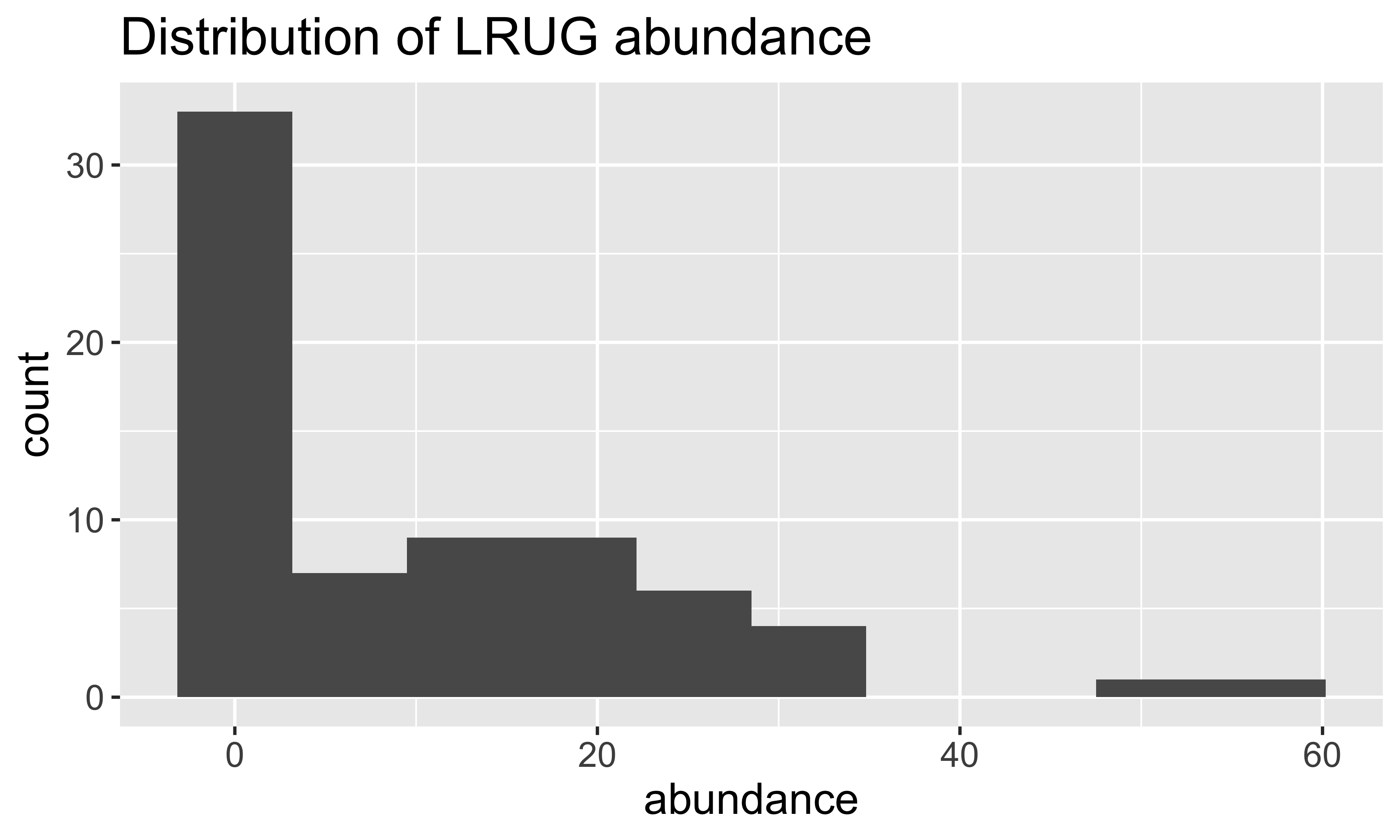
# Focus on just the LRUG mite abundances
mite_dat <- mite.env %>%
add_column(abundance = mite$LRUG)
head(mite_dat) SubsDens WatrCont Substrate Shrub Topo abundance
1 39.18 350.15 Sphagn1 Few Hummock 0
2 54.99 434.81 Litter Few Hummock 0
3 46.07 371.72 Interface Few Hummock 0
4 48.19 360.50 Sphagn1 Few Hummock 0
5 23.55 204.13 Sphagn1 Few Hummock 0
6 57.32 311.55 Sphagn1 Few Hummock 0EDA
(scroll for more content)
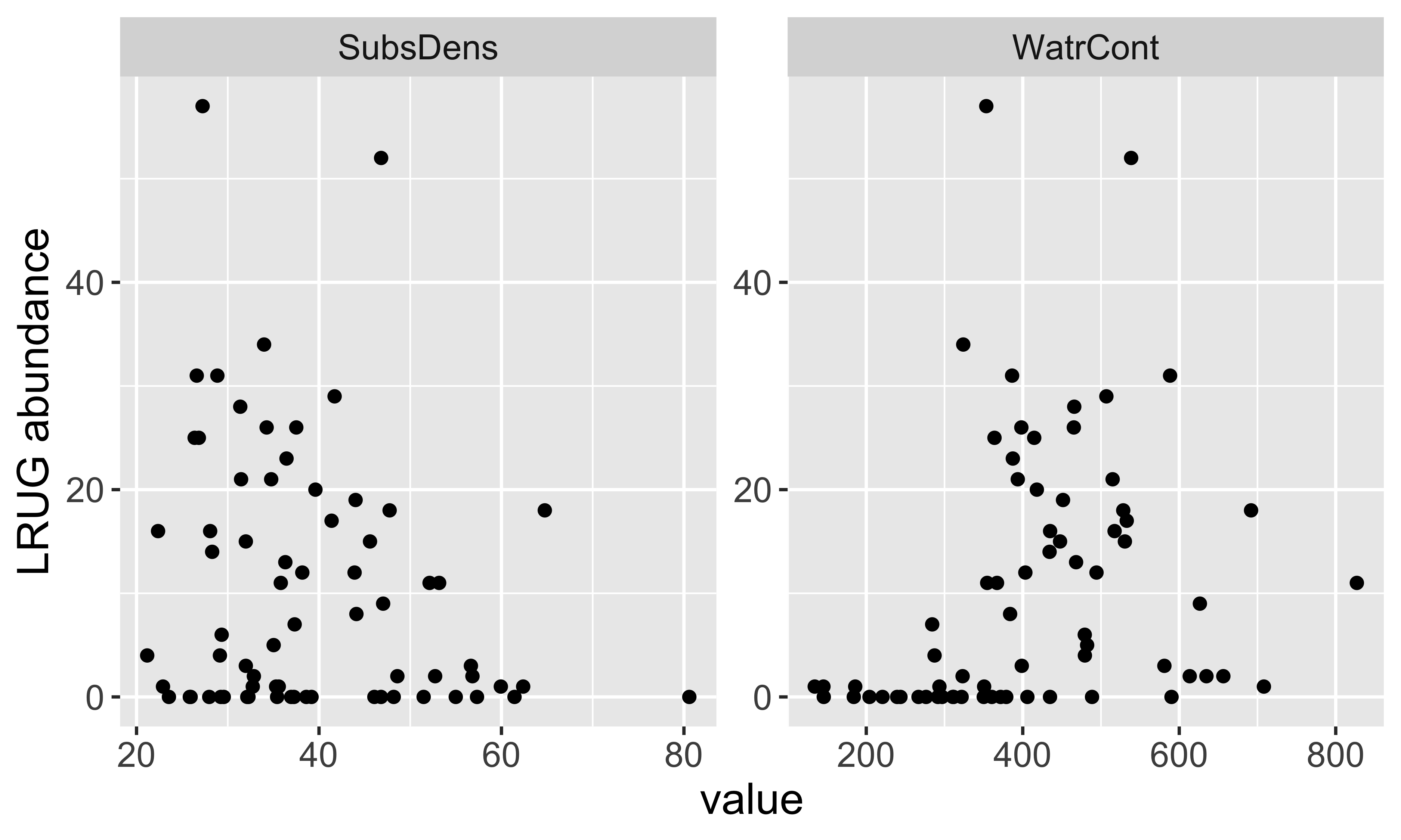
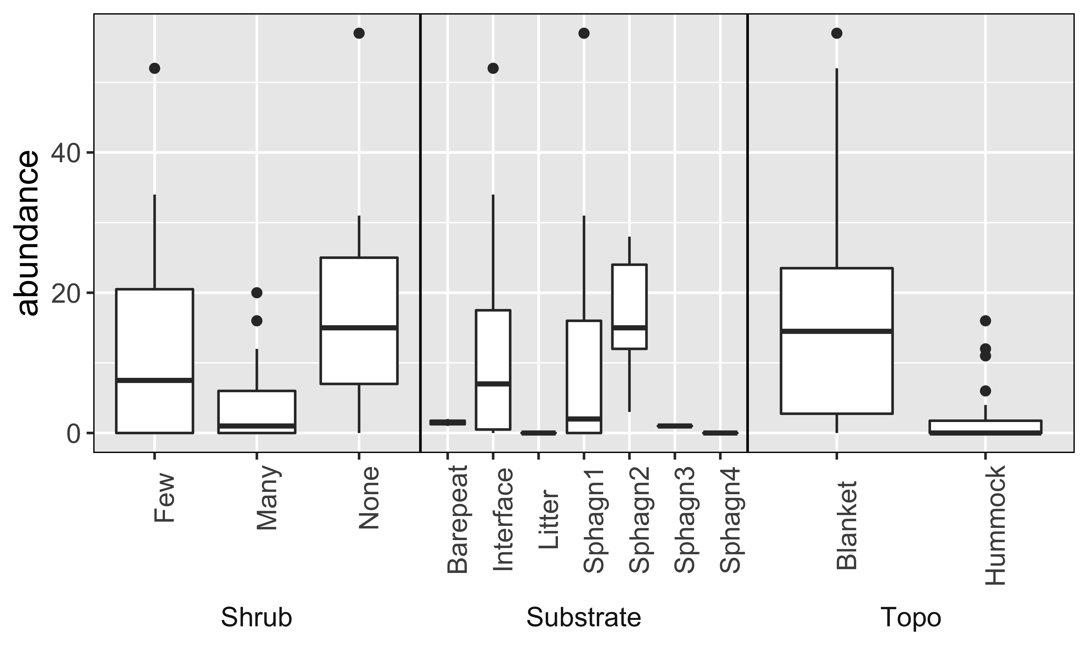
Statistical learning tasks
Model building
Goal: predict
LRUGabundance using these variablesMaybe
LRUG\(\approx f(\)SubsDens+WatrCont\()\)?If so, how would we represent these variables using our notation? i.e., what are \(y_{i}\) and \(x_{i}\)?
Then our model can be written as \(y_{i} = f(x_{i}) + \epsilon_{i}\) where \(\epsilon_{i}\) represents random measurement error
What does this equation mean?
Why care about f?
Model (dropping the indices): \(Y = f(X) + \epsilon\)
The function \(f(X)\) represents the systematic information that \(X\) tells us about \(Y\).
If \(f\) is “good”, then we can make reliable predictions of \(Y\) at new points \(X = x\)
If \(f\) is “good”, then we can identify which components of \(X\) are important for explaining \(Y\)
- Depending on \(f\), we may be able to learn how each component of \(X\) affects \(Y\)
Why care about f?
- We assume that \(f\) is fixed but unknown
- Goal of statistical learning: how to obtain an estimate \(\hat{f}\) of the true \(f\)?
- Sub-goals: prediction and inference
- The sub-goal may affect our choice of \(\hat{f}\)
Prediction
We have a set of inputs or predictors \(x_{i}\), and we want to predict a corresponding \(y_{i}\). Assume the true model is \(y_{i} = f(x_{i}) + \epsilon_{i}\), but don’t know \(f\)
Assuming the error \(\epsilon_{i}\) is 0 on average, we can obtain predictions of \(y_{i}\) as \[\hat{y}_{i} = \hat{f}(x_{i})\]
- Then, if we know the true \(y_{i}\), we can evaluate the accuracy of the prediction \(\hat{y}_{i}\)
Generally, \(y_{i} \neq \hat{y}_{i}\). Why?
- \(\hat{f}\) will not be perfect estimate of \(f\)
- \(y_{i}\) is a function of \(\epsilon_{i}\), which cannot be predicted using \(x_{i}\)
Types of error
Model: \(y_{i} = f(x_{i}) + \epsilon_{i}\)
Irreducible error: \(\epsilon_{i}\)
- Even if we knew \(f\) perfectly, there is still some inherent variability
- \(\epsilon_{i}\) may also contain unmeasured variables that are not available to us
Reducible error: how far \(\hat{f}\) is from the true \(f\)
Prediction errors
- Ways to quantify error
- Difference/error = \(y_{i} - \hat{y}_{i}\)
- Absolute error = \(|y_{i} - \hat{y}_{i}|\)
- Squared error = \((y_{i} - \hat{y}_{i})^2\)
- Intuitively, larger error indicates worse prediction
- Question: are there scenarios where we might prefer one error over another?
Prediction errors
Given \(\hat{f}\) and \(x_{i}\), we can obtain a prediction \(\hat{y}_{i} = \hat{f}(x_{i})\) for \(y_{i}\)
Mean-squared prediction error: \[\begin{align*} \mathsf{E}[(y_{i} - \hat{y}_{i})^2] &= \mathsf{E}[( f(x_{i}) + \epsilon_{i} - \hat{f}(x_{i}))^2] \\ &= \underbrace{[f(x_{i}) - \hat{f}(x_{i})]^2}_\text{reducible} + \underbrace{\text{Var}(\epsilon_{i})}_\text{irreducible} \end{align*}\]
We cannot do much to decrease the irreducible error
But we can potentially minimize the reducible error by choosing better \(\hat{f}\)!
Inference
- We are often interested in learning how \(Y\) and the \(X_{1}, \ldots, X_{p}\) are related or associated
- In this mindset, we want to estimate \(f\) to learn the relationships, rather than obtain a \(\hat{Y}\)
Prediction vs Inference
Prediction: estimate \(\hat{f}\) for the purpose of \(\hat{Y}\) and \(Y\).
Inference: estimate \(\hat{f}\) for the purpose of \(X\) and \(Y\)
Some problems will call for prediction, inference, or both
To what extent is
LRUGabundance associated withmicrotopography?Given a specific land profile, how many
LRUGmites would we expect there to be?
Assessment
Assessing model accuracy
No single method or choice of \(\hat{f}\) is superior over all possible data sets
Prediction accuracy vs. interpretability
More restrictive models may be easier to interpret (better for inference)
Good fit vs. over-fit (or under-fit)
A simpler model is often preferred over a very complex one
Assessing model accuracy
How can we know how well a chosen \(\hat{f}\) is performing?
In regression setting, we often use mean squared error (MSE) or root MSE (RMSE)
\(\text{MSE}=\frac{1}{n}\sum_{i=1}^{n}(y_{i}-\hat{f}(x_{i}))^2\)
\(\text{RMSE}=\sqrt{\frac{1}{n}\sum_{i=1}^{n}(y_{i}-\hat{f}(x_{i}))^2}\)
MSE (and RMSE) will be small if predictions \(\hat{y}_{i} = \hat{f}(x_{i})\) are very close to true \(y_{i}\)
Question: why might we prefer reporting RMSE over MSE?
Training vs. test data
In practice, we split our data into training and test sets
- Training set is used to fit the model
- Test set is used to assess model fit
We are often most interested in accuracy of our predictions when applying the method to previously unseen data. Why?
We can compute the MSE for the training and test data respectively…but we typically focus more attention to test MSE
Example 1
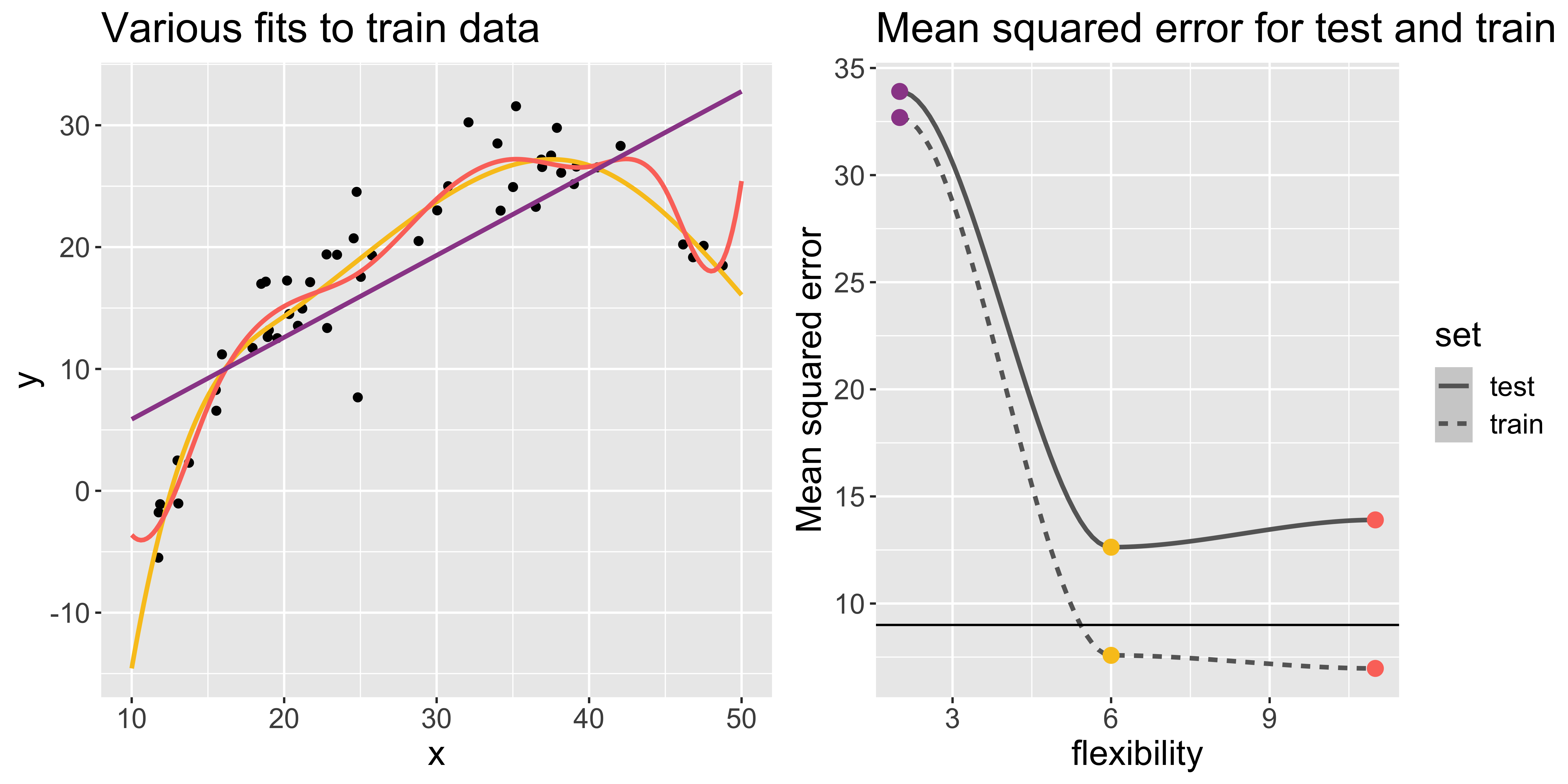
I generated some fake data and fit three models that differ in flexibility. In this example, the generated data (points) follow a curve-y shape.
Example 2
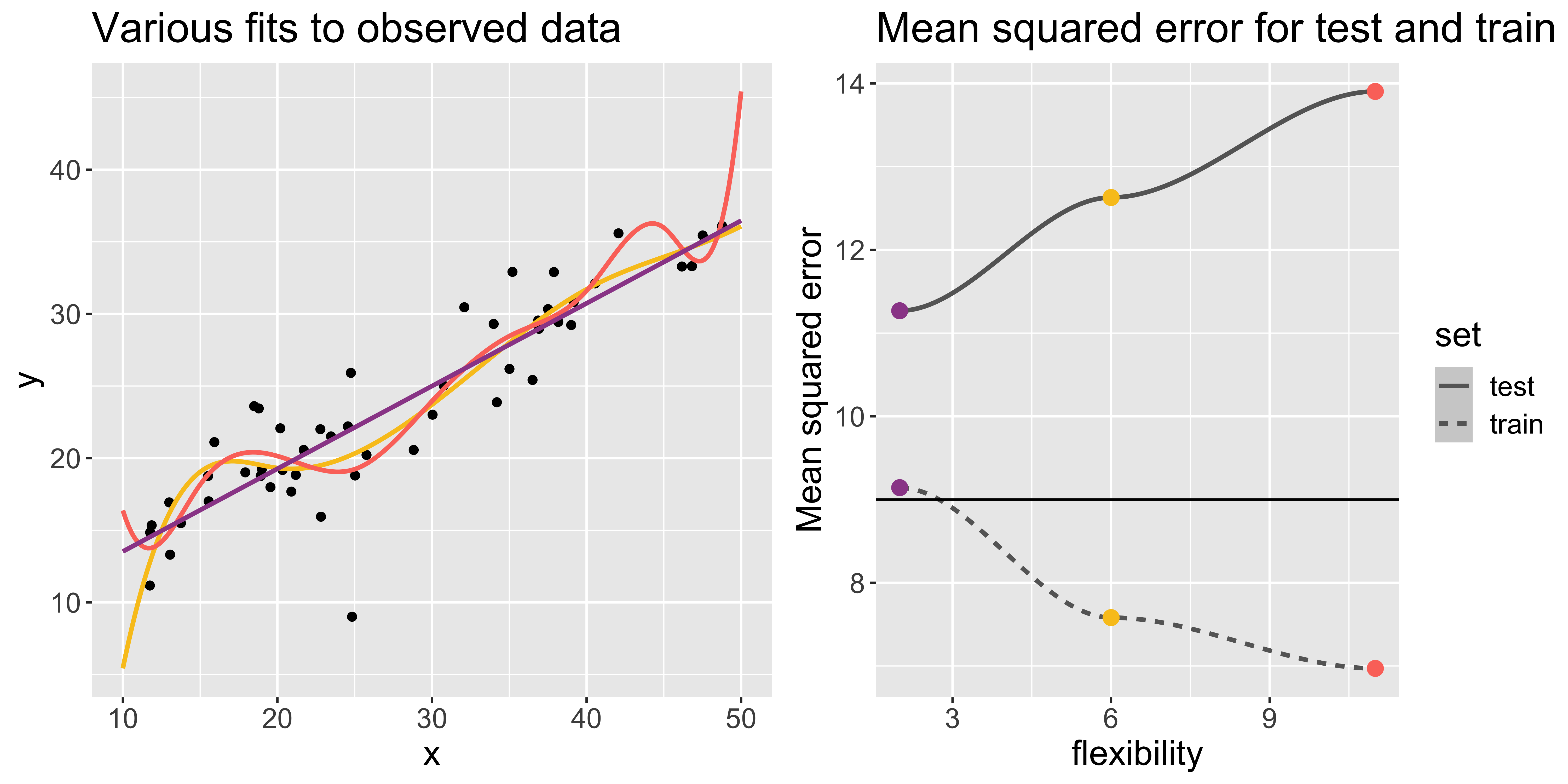
In this example, the generated data (points) look more linear.
Bias-Variance trade-off
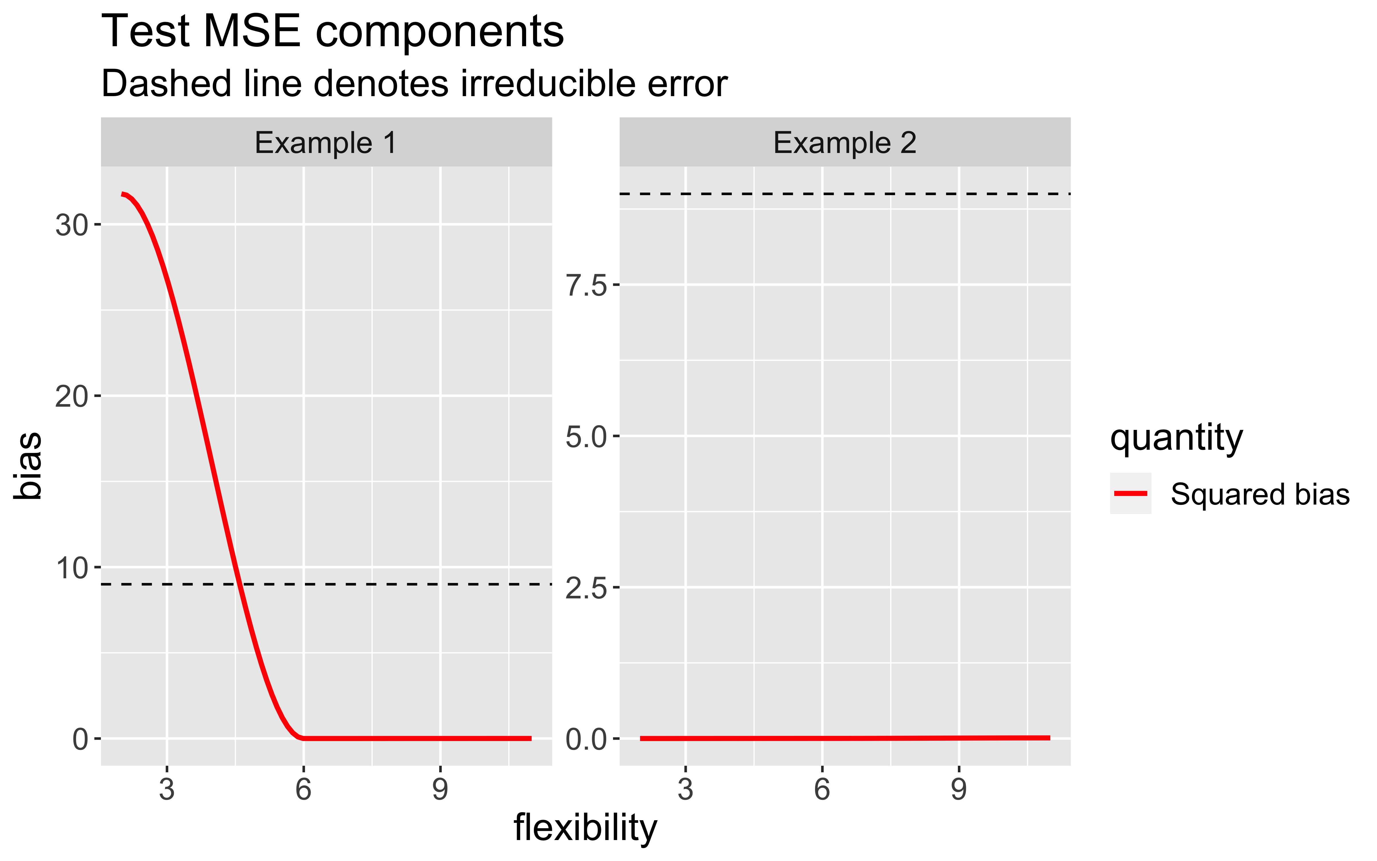
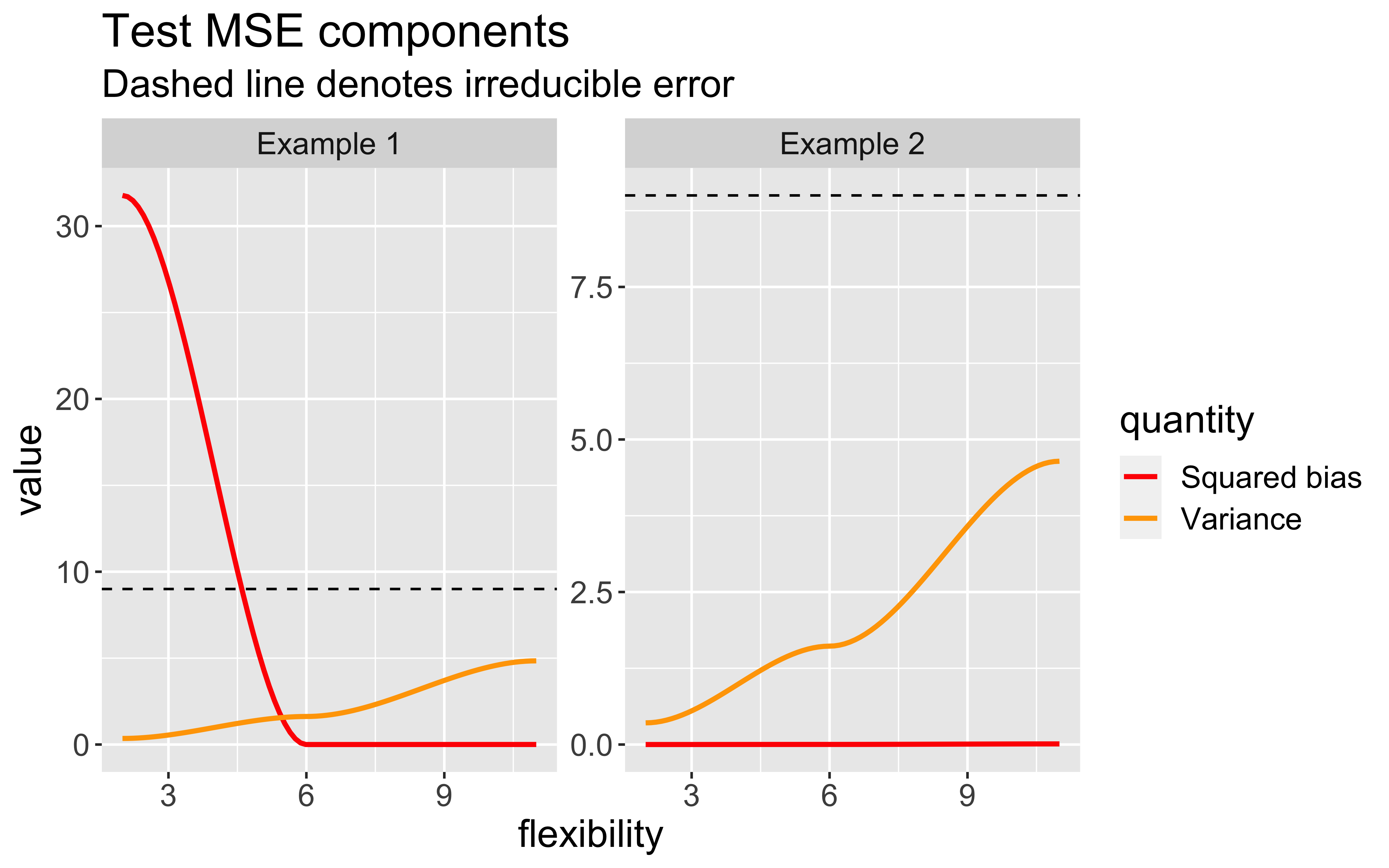
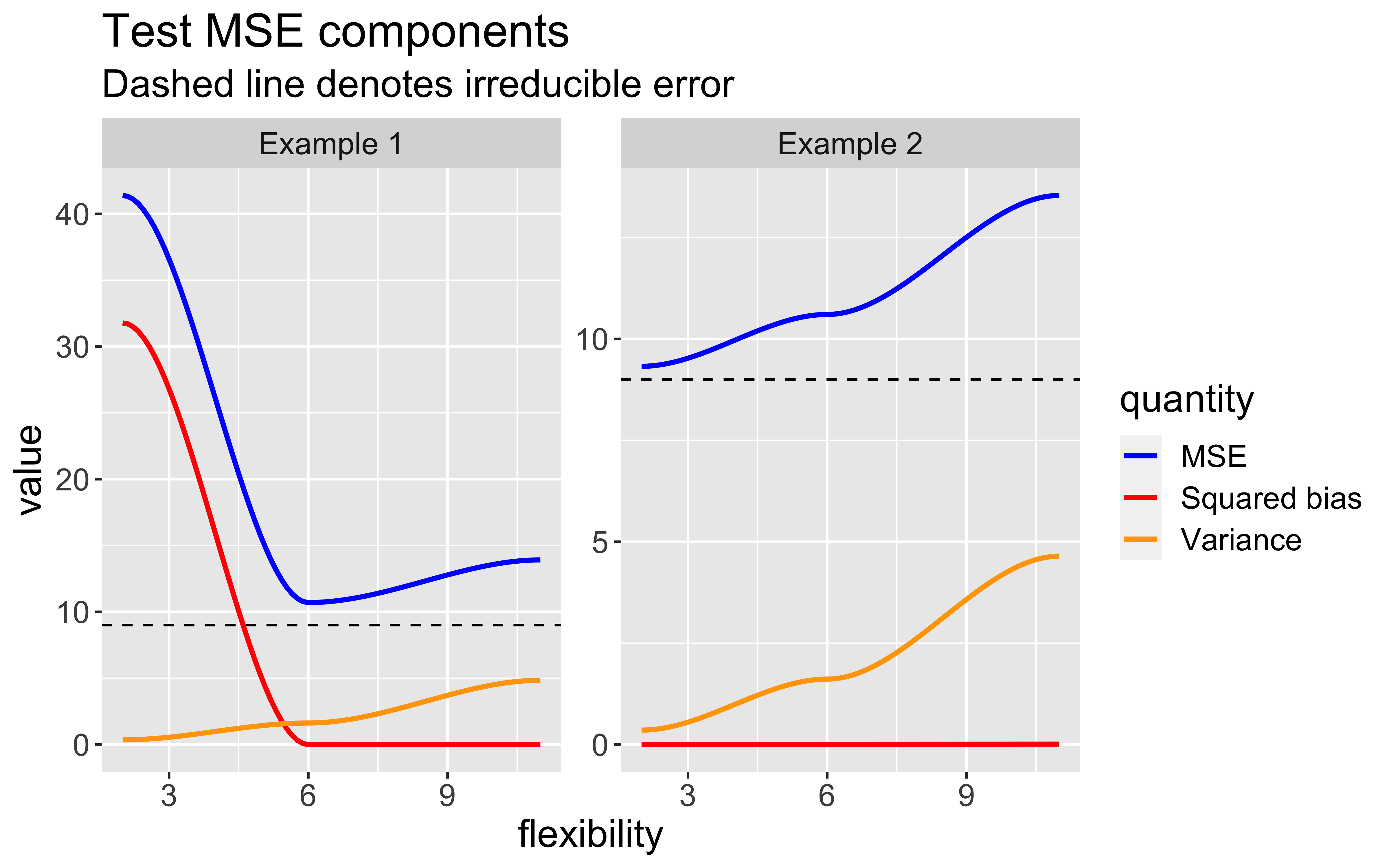
As model flexibility increases, the training MSE will decrease but test MSE may not.
Flexible models may overfit the data, which leads to low train MSE and high test MSE
- The supposed patterns in train data do not exist in test data
Let us consider a test observation \((x_{0}, y_{0})\).
The expected test MSE for given \(x_{0}\) can be decomposed as follows:
\(\mathsf{E}[(y_{0} - \hat{f}(x_{0}))^2] = \text{Var}(\hat{f}(x_{0})) + [\text{Bias}(\hat{f}(x_{0}))]^2 + \text{Var}(\epsilon)\)
\(\text{Bias}(\hat{f}(x_{0})) = \mathsf{E}[\hat{f}(x_{0})] - \hat{f}(x_{0})\)
Bias-Variance trade-off (cont.)
