Live code:
Mini implementation
We will write code to understand how recursive binary splitting works. Specifically, we will pretend we are about to create the root node (i.e. first split) for a regression tree that uses WatrCont and SubsDens to predict abundance of the mites. We need to obtain the residual sum of squares (RSS) for each candidate split, and choose the split that yields the best (lowest) RSS at that step in the tree, where RSS is
\[\sum_{i:x_{i}\in S_l(j,c)} (y_{i} - \hat{y}_{S_{l}})^2 + \sum_{i:x_{i}\in S_r(j,c)} (y_{i} - \hat{y}_{S_{r}})^2,\]
and \(\hat{y}_{S_{l}}\) is the average of the training responses in \(S_l(j,s)\)
So from this, we need to:
- Determine if each observation goes left or right based on the condition
- Obtain the average of the training responses in each side (\(\hat{y}_{S_{l}}\) and \(\hat{y}_{S_{r}}\))
- Obtain the residual of each observation
- Obtain the RSS from each set \(S_{l}\) and \(S_{r}\)
- Obtain one single RSS, which is the sum of the two values in (4)
We saw that one candidate split was SubsDens < 22.63. Let’s see what the resulting RSS is from this split.
Make sure you understand what each line of code is doing. If not, please ask!
mite_dat%>%
  mutate(decision = if_else(SubsDens < 22.63, "left", "right")) %>%
  group_by(decision) %>%
  mutate(y_hat = mean(abundance)) %>%
  ungroup() %>%
  mutate(sq_resid = (abundance - y_hat)^2) %>%
  group_by(decision) %>%
  summarise(rss = sum(sq_resid)) %>%
  pull(rss) %>%
  sum()
[1] 11058.76If instead we considered the candidate split WatrCont < 145.48:
mite_dat%>%
  mutate(decision = if_else(WatrCont < 145.48, "left", "right")) %>%
  group_by(decision) %>%
  mutate(y_hat = mean(abundance)) %>%
  ungroup() %>%
  mutate(sq_resid = (abundance - y_hat)^2) %>%
  group_by(decision) %>%
  summarise(rss = sum(sq_resid)) %>%
  pull(rss) %>%
  sum()
[1] 10876.12Notice that we get a different candidate RSS!
Coding in R
trees() function
Simple regression trees can be implemented in R using the trees library (you may have to install) using the tree() function. The syntax is just as in lm():
Note: the tree() function we will use requires all categorical variables to be coded as factors. Additionally, no single categorical variable can have more than 32 levels.
library(tree)

tree_mites <- tree(abundance ~ WatrCont + SubsDens + Topo,

                   data = mite_dat)

summary(tree_mites)
Regression tree:
tree(formula = abundance ~ WatrCont + SubsDens + Topo, data = mite_dat)
Number of terminal nodes:  8
Residual mean deviance:  64.95 = 4027 / 62
Distribution of residuals:
    Min.  1st Qu.   Median     Mean  3rd Qu.     Max.
-23.0000  -3.3590  -0.8571   0.0000   2.4890  28.3300
Above, lines 2-3 fit the regression trees for abundance using the three specified predictors from mite_dat data. Similar to lm(), we can wrap the tree object with summary() to get some more information about the model fit. We see number of terminal notes \(|T_{0}|\), the predictors that were used to build the tree, and residual mean deviance:
If you don’t see list of predictors, then the tree used all of them
Residual mean deviance: \(\text{RSS}/(n - |T_{0}|)\)
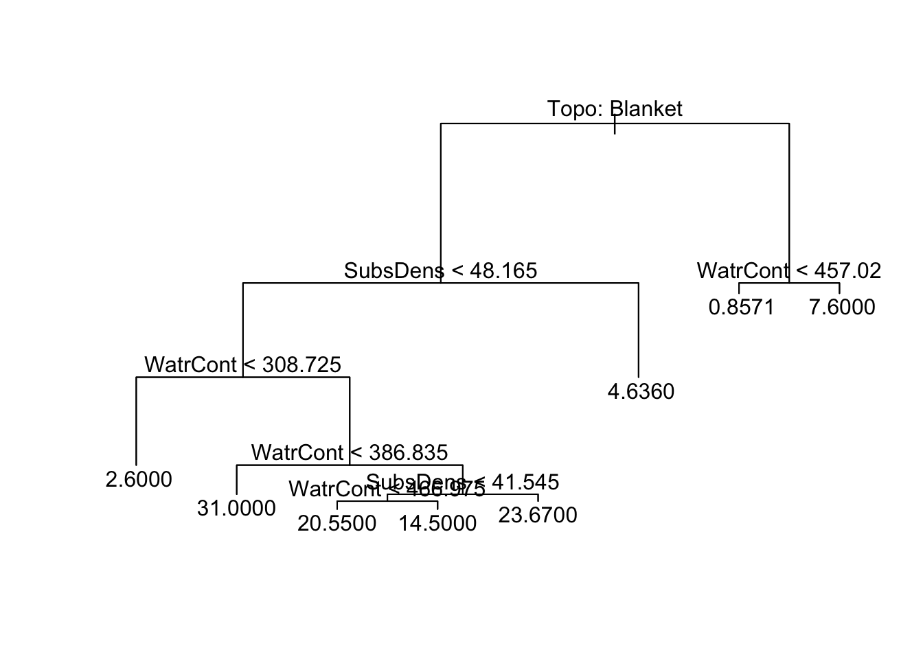
Typing the name of the tree object prints the tree in text form:
node), split, n, deviance, yval
      * denotes terminal node

 1) root 70 11060.0 10.4300
   2) Topo: Blanket 44  7760.0 15.3200
     4) SubsDens < 48.165 33  5734.0 18.8800
       8) WatrCont < 308.725 5    33.2  2.6000 *
       9) WatrCont > 308.725 28  4139.0 21.7900
        18) WatrCont < 386.835 5  1250.0 31.0000 *
        19) WatrCont > 386.835 23  2372.0 19.7800
          38) SubsDens < 41.545 17  1074.0 18.4100
            76) WatrCont < 466.975 11   308.7 20.5500 *
            77) WatrCont > 466.975 6   623.5 14.5000 *
          39) SubsDens > 41.545 6  1175.0 23.6700 *
     5) SubsDens > 48.165 11   352.5  4.6360 *
   3) Topo: Hummock 26   467.4  2.1540
     6) WatrCont < 457.02 21   120.6  0.8571 *
     7) WatrCont > 457.02 5   163.2  7.6000 *
We can interpret the tree as follows:
The * denotes a terminal node
split: condition used to branch at the noden: the number of observations following the left-side of the branchdeviance: the deviance associated with that branchyval: predicted value at the node
Plotting trees
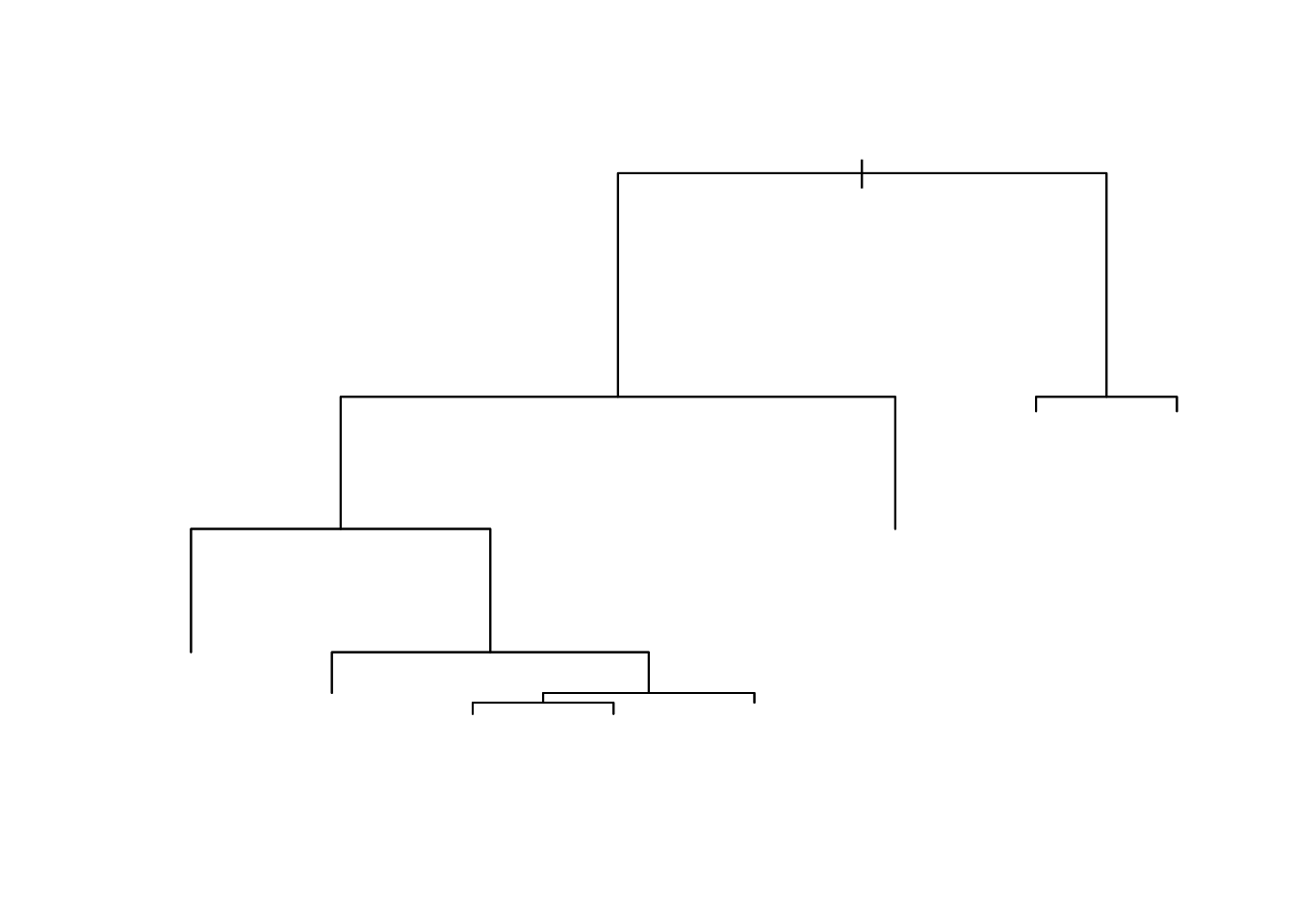
We will use base R plots; I’m sure there are much more beautiful ggplot functions out there, but I’m not in the business of it today! We simply pass the tree object into plot():
Notice that there is no text! This isn’t helpful. We need to explicitly add the labels using the text() function:
The argument pretty = 0 instructs R to include the category names for any qualitative predictors, rather than simply displaying a generic a, b, c… letter for each category.
If you get an error when trying to use text(), it’s because text() doesn’t like it when your plot shows up inline. This shouldn’t be an issue when you knit. If you want to see your tree without knitting, go to the gear symbol at the top of the Rmarkdwon document, hit the down arrow, then hit “Chunk output in Console”. You’ll be prompted if you want to remove the current output (yes or not are both fine!) Then try running the code again.

