Live code:

Hierarchical clustering

hclust()

library(tidyverse)

We use the function hclust() to implement hierarchical clustering! We need to pass in two arguments:

• A distance matrix of the dissimilarities between observations. The distance matrix must always be \(n \times n\), where \(n\) is the number of observations. The pairwise Euclidean distances are easily calculated used dist().

• We also need to specify the type of linkage, in quotes

  • “average”, “single”, “complete”, or “centroid” (there are others, but we didn’t discuss in class)

We will visit the USArrests data we saw in class. I will grab two variables, and go ahead and standardize them.

data("USArrests")
usarrests <- USArrests %>%
  select(Murder, UrbanPop) %>%
  mutate_all(scale)

dists <- dist(usarrests)
hc_complete <- hclust(d = dists, method = "complete")

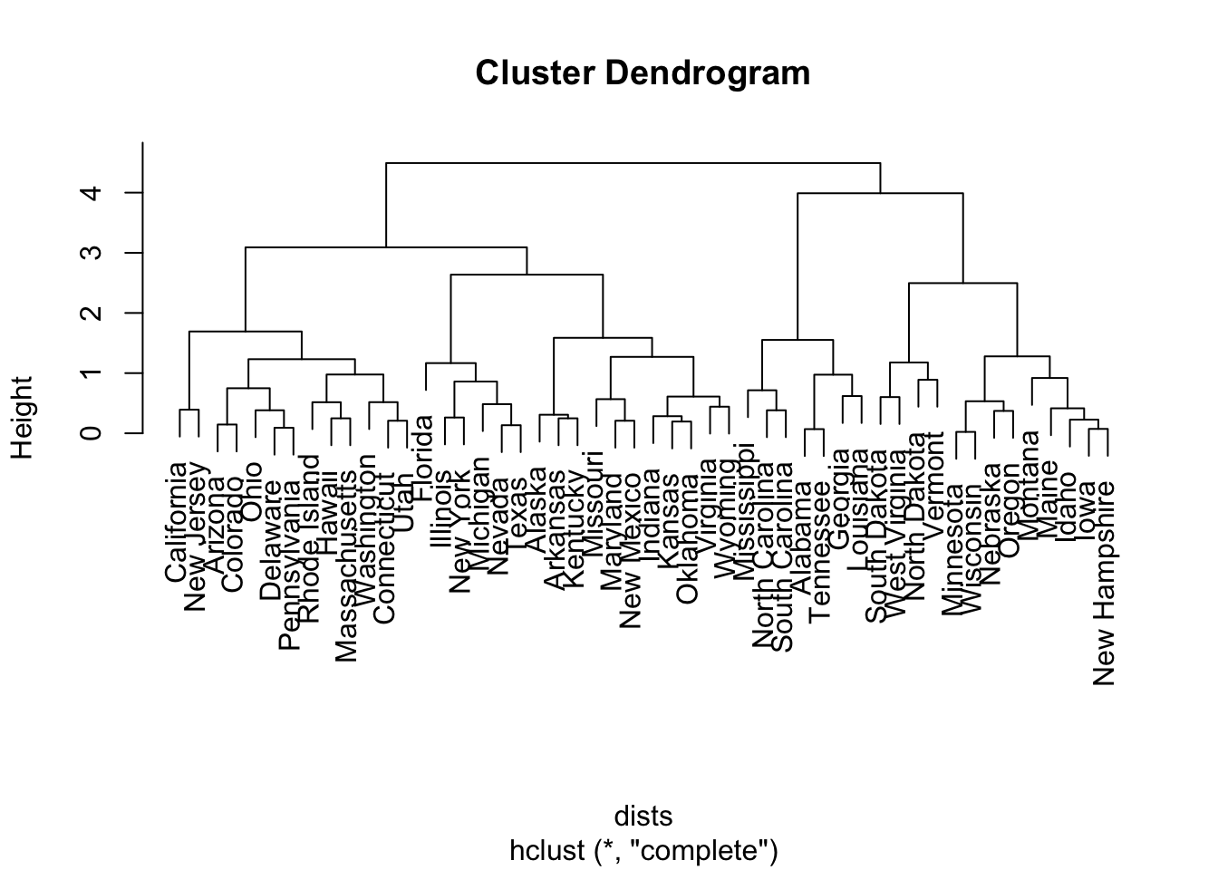
We can easily pass the output into the plot() function to visualize the entire dendrogram:

plot(hc_complete)

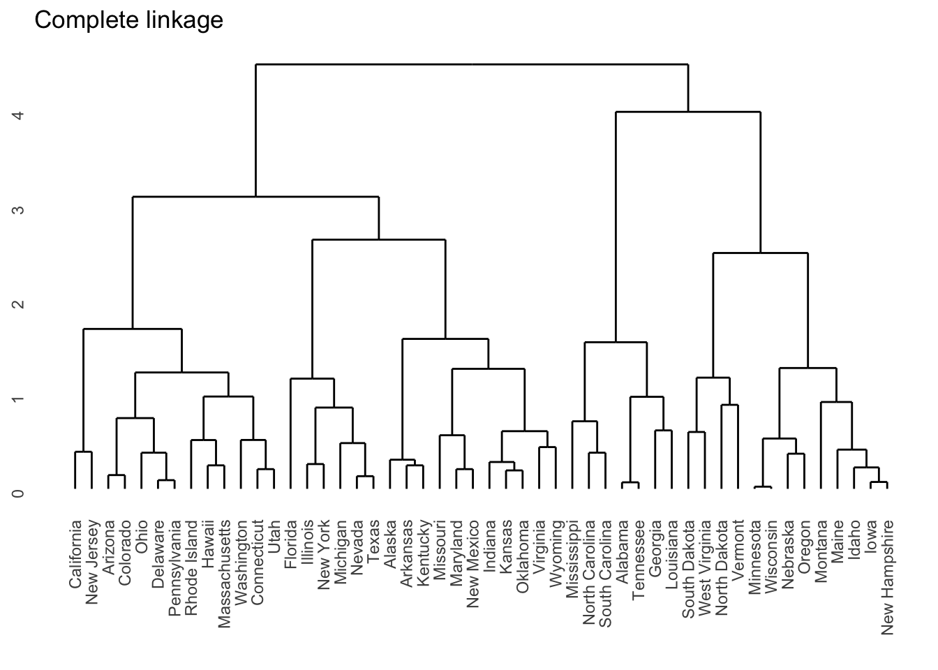
I personally prefer ggplots, so if you install the ggdendro package, you can obtain the following plot:

library(ggdendro)
ggdendrogram(hc_complete) +
  ggtitle("Complete linkage")

To determine the cluster labels associated with a given cut of the dendrogram, we use the cutree() function. It takes in the output from hclust() and the number of clusters k we want to obtain. In the following, I obtain three clusters:

k <- 3
hclusts <- cutree(hc_complete, k = k)
hclusts

       Alabama         Alaska        Arizona       Arkansas     California 
             1              2              2              2              2 
      Colorado    Connecticut       Delaware        Florida        Georgia 
             2              2              2              2              1 
        Hawaii          Idaho       Illinois        Indiana           Iowa 
             2              3              2              2              3 
        Kansas       Kentucky      Louisiana          Maine       Maryland 
             2              2              1              3              2 
 Massachusetts       Michigan      Minnesota    Mississippi       Missouri 
             2              2              3              1              2 
       Montana       Nebraska         Nevada  New Hampshire     New Jersey 
             3              3              2              3              2 
    New Mexico       New York North Carolina   North Dakota           Ohio 
             2              2              1              3              2 
      Oklahoma         Oregon   Pennsylvania   Rhode Island South Carolina 
             2              3              2              2              1 
  South Dakota      Tennessee          Texas           Utah        Vermont 
             3              1              2              2              3 
      Virginia     Washington  West Virginia      Wisconsin        Wyoming 
             2              2              3              3              2 

From the output, we can see to which of the 4 clusters each state has been assigned. To get an idea of the spread across the clusters, we can use the table() function:

table(hclusts)

hclusts
 1  2  3 
 7 30 13 

Comparing to k-means

What happens if I run the k-means algorithm on the same set of data? Do we think the two methods will agree with each other if I specify I want the same number of clusters?

set.seed(1)
kmeans_out <- kmeans(usarrests, centers = k, nstart = 10)
kmeans_clusts <- kmeans_out$cluster

Now, let’s be careful! There’s no reason why cluster 1 from hierarchical clustering should be the “same” as cluster 1 from k-means. So if we want to compare the results from the two methods, we just need to see if a cluster from the hierarchical method has a lot of the same observations as a cluster from k-means.

table(hclusts, kmeans_clusts)

       kmeans_clusts
hclusts  1  2  3
      1  0  0  7
      2  1 21  8
      3 12  1  0

Linkage choices

Try playing around with different choices of linkage! What do you notice if you use single linkage?