Live code:

Bagging trees

library(tidyverse)
library(vegan)
library(randomForest)
data(mite)
data(mite.env)
mite_dat <- mite.env %>%
  add_column(abundance = mite$LRUG)

Introduction

We will use the R package called randomForest is fit bagged decision trees and random forests. Go ahead and install this package in your console!

As we will see in the slides, bagged trees and random forests are very similar and can be fit using the same function: randomForest(). The difference lies in the specification of the mtry argument, as we will see below.

Bagging

The syntax for bagged regression trees is the same as in regular regression trees: response ~ predictors.

In bagged regression trees, the only parameter that the modeler needs to choose is the number of bootstrap samples \(B\) to obtain (and therefore the number of trees to fit). This is denoted as the ntree argument

However, we will need to specify the additional mtry argument to specify we want to fit a bagged model rather than a random forest. For bagged trees, we set mtry equal to the number of predictors we have.

In the following code, I fit B = 10 regression trees, and specify mtry = 5.

set.seed(2)
n <- nrow(mite_dat)
train_ids <- sample(1:n, 0.8*n)
bag_mod <- randomForest(abundance ~ . , data = mite_dat[train_ids,],
                    ntree = 10, 
                    mtry = ncol(mite_dat) - 1)

To make predictions for the test set, we will use the familiar predict() function:

preds <- predict(bag_mod, newdata = mite_dat[-train_ids,])
preds

       10        14        20        21        24        25        26        29 
 0.400000  3.675000  0.700000  5.916667  0.400000  4.125000  6.050000  4.166667 
       31        37        46        52        63        66 
 9.240000 24.790000 21.910000 16.800000 19.616667 23.231667 

Out-of-bag error

The nice thing about bootstrapping is that typically ~1/3 of observations are left out in each sample (and therefore, in each one of the B trees). So, we don’t necessarily need to explicitly specify a test/train split!

In the following code, a fit a bagged model using all of the available observations:

set.seed(5)
bag_all <- randomForest(abundance ~ . , data = mite_dat,
                    ntree = 10, 
                    mtry = ncol(mite_dat) - 1)

The randomForest() function will automatically create a vector of predicted values for the input data based on the out of bag (OOB) samples; i.e. whenever observation \(i\) is OOB (not included in the bootstrap sample) for tree \(b\), we can treat \(i\) as a test observation and obtain a prediction for it. This is accessed through the predicted component of the fitted model:

bag_all$predicted

          1           2           3           4           5           6 
 3.86666667  5.27777778  8.30000000  3.75833333  0.00000000  0.31111111 
          7           8           9          10          11          12 
 3.61944444  2.79000000  0.60000000  0.15000000  2.00000000  0.88888889 
         13          14          15          16          17          18 
 0.00000000  5.92500000 33.70000000  2.06250000  1.52777778  0.66666667 
         19          20          21          22          23          24 
32.80000000  1.37500000  4.56250000  0.08571429 12.01111111  2.31250000 
         25          26          27          28          29          30 
 0.40000000  7.05555556  0.65000000  7.80000000  0.30000000 19.75000000 
         31          32          33          34          35          36 
 4.58333333  0.13333333 21.30000000 16.61000000          NA  9.14285714 
         37          38          39          40          41          42 
14.99000000 11.75000000  1.00000000 21.10000000 24.82000000 22.60000000 
         43          44          45          46          47          48 
 9.70833333  5.86666667 13.41666667 14.50000000  1.40000000 11.31000000 
         49          50          51          52          53          54 
44.11666667 13.25000000 16.25000000 16.81250000 18.13333333 17.58333333 
         55          56          57          58          59          60 
19.22000000 16.25000000  2.03666667 11.86666667  7.67000000 20.80000000 
         61          62          63          64          65          66 
19.06666667 13.40714286 15.03333333 19.32857143 14.75000000 15.45000000 
         67          68          69          70 
 6.20000000 34.00000000  4.54666667  3.50000000 

Do you notice anything strange in these predictions?

Importance measure

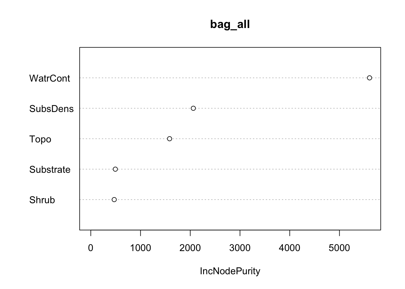
In order to obtain a measure of how “important” each predictor is by accessing the importance component. For regression tasks, this corresponds to the total amount that MSE decreases due to splits over a predictor, averaged over B:

bag_all$importance

          IncNodePurity
SubsDens      2061.6646
WatrCont      5604.9744
Substrate      493.4425
Shrub          470.8712
Topo          1584.0990

importance(bag_all)

          IncNodePurity
SubsDens      2061.6646
WatrCont      5604.9744
Substrate      493.4425
Shrub          470.8712
Topo          1584.0990

We can use the varImpPlot() function to visualize the importance:

varImpPlot(bag_all)

Random Forests

The syntax for random forests is almost identical to that of bagging regression trees. Unlike bagging, we need to specify two parameters for random forests:

1. The number of bootstrap samples \(B\) to obtain (as in bagging)
2. The number of predictors we should consider at each split (i.e. the mtry argument)

In the following code, I fit B = 10 regression trees, and specify mtry = 2.

set.seed(1)
rf_mod <- randomForest(abundance ~ . , data = mite_dat,
                    ntree = 10, 
                    mtry = 2)

Everything else is exactly the same as in bagged regression trees!